EMC² Demo Notebook
In this notebook we show an example of how to run \(EMC^2\) using ModelE3 climate model output and high spectral resolution lidar (HSRL) data, and demonstrate some of the framework’s plotting capabilities.
[1]:
import emc2
import matplotlib.dates as mdates
First, we load model data (in this case, ModelE3) using the ModelE subclass object
[2]:
model_path = 'allsteps.allmergeSCM_AWARE_788.nc'
my_model = emc2.core.model.ModelE(model_path)
After that, we load in the HSRL data using the HSRL subclass object.
[3]:
HSRL = emc2.core.instruments.HSRL('nsa')
HSRL.read_arm_netcdf_file('awrhsrlM1.20160816.100000.nc')  # raw or processed ARM or ARM-like data file
[4]:
HSRL.ds
[4]:
<xarray.Dataset>
Dimensions:                                (time: 120, mean_time: 120,
                                            altitude: 334, profile_time: 1)
Coordinates:
  * time                                   (time) datetime64[ns] 2016-08-16T1...
  * mean_time                              (mean_time) object 2016-08-16 10:0...
  * altitude                               (altitude) float32 0.0 ... 9.99e+03
Dimensions without coordinates: profile_time
Data variables: (12/26)
    base_time                              object ...
    first_time                             object ...
    last_time                              object ...
    latitude                               (time) float32 dask.array<chunksize=(120,), meta=np.ndarray>
    longitude                              (time) float32 dask.array<chunksize=(120,), meta=np.ndarray>
    od                                     (time, altitude) float32 dask.array<chunksize=(120, 334), meta=np.ndarray>
    ...                                     ...
    profile_beta_a_backscat_parallel       (profile_time, altitude) float32 dask.array<chunksize=(1, 334), meta=np.ndarray>
    beta_a_backscat_perpendicular          (time, altitude) float32 dask.array<chunksize=(120, 334), meta=np.ndarray>
    profile_beta_a_backscat_perpendicular  (profile_time, altitude) float32 dask.array<chunksize=(1, 334), meta=np.ndarray>
    beta_a_backscat                        (time, altitude) float32 dask.array<chunksize=(120, 334), meta=np.ndarray>
    profile_beta_a_backscat                (profile_time, altitude) float32 dask.array<chunksize=(1, 334), meta=np.ndarray>
    qc_mask                                (time, altitude) float64 dask.array<chunksize=(120, 334), meta=np.ndarray>
Attributes: (12/94)
    dpl_py_template:                                                         ...
    dpl_py_template_version:                                                 ...
    time_zone:                                                               ...
    codeversion:                                                             ...
    codedate:                                                                ...
    hsrl_instrument:                                                         ...
    ...                                                                                   ...
    hsrl_processing_parameter__wfov_corr__window_durration:                  ...
    hsrl_processing_parameter__wfov_corr__z_norm_interval:                   ...
    _file_dates:                                                             ...
    _file_times:                                                             ...
    _datastream:                                                             ...
_arm_standards_flag: ...- time: 120
- mean_time: 120
- altitude: 334
- profile_time: 1
- time(time)datetime64[ns]2016-08-16T10:00:00 ... 2016-08-...
- long_name :
- Time
- dpl_py_binding :
- rs_inv.times
- dpl_py_type :
- python_datetime
array(['2016-08-16T10:00:00.000000000', '2016-08-16T10:00:30.000000000', '2016-08-16T10:01:00.000000000', '2016-08-16T10:01:30.000000000', '2016-08-16T10:02:00.000000000', '2016-08-16T10:02:30.000000000', '2016-08-16T10:03:00.000000000', '2016-08-16T10:03:30.000000000', '2016-08-16T10:04:00.000000000', '2016-08-16T10:04:30.000000000', '2016-08-16T10:05:00.000000000', '2016-08-16T10:05:30.000000000', '2016-08-16T10:06:00.000000000', '2016-08-16T10:06:30.000000000', '2016-08-16T10:07:00.000000000', '2016-08-16T10:07:30.000000000', '2016-08-16T10:08:00.000000000', '2016-08-16T10:08:30.000000000', '2016-08-16T10:09:00.000000000', '2016-08-16T10:09:30.000000000', '2016-08-16T10:10:00.000000000', '2016-08-16T10:10:30.000000000', '2016-08-16T10:11:00.000000000', '2016-08-16T10:11:30.000000000', '2016-08-16T10:12:00.000000000', '2016-08-16T10:12:30.000000000', '2016-08-16T10:13:00.000000000', '2016-08-16T10:13:30.000000000', '2016-08-16T10:14:00.000000000', '2016-08-16T10:14:30.000000000', '2016-08-16T10:15:00.000000000', '2016-08-16T10:15:30.000000000', '2016-08-16T10:16:00.000000000', '2016-08-16T10:16:30.000000000', '2016-08-16T10:17:00.000000000', '2016-08-16T10:17:30.000000000', '2016-08-16T10:18:00.000000000', '2016-08-16T10:18:30.000000000', '2016-08-16T10:19:00.000000000', '2016-08-16T10:19:30.000000000', '2016-08-16T10:20:00.000000000', '2016-08-16T10:20:30.000000000', '2016-08-16T10:21:00.000000000', '2016-08-16T10:21:30.000000000', '2016-08-16T10:22:00.000000000', '2016-08-16T10:22:30.000000000', '2016-08-16T10:23:00.000000000', '2016-08-16T10:23:30.000000000', '2016-08-16T10:24:00.000000000', '2016-08-16T10:24:30.000000000', '2016-08-16T10:25:00.000000000', '2016-08-16T10:25:30.000000000', '2016-08-16T10:26:00.000000000', '2016-08-16T10:26:30.000000000', '2016-08-16T10:27:00.000000000', '2016-08-16T10:27:30.000000000', '2016-08-16T10:28:00.000000000', '2016-08-16T10:28:30.000000000', '2016-08-16T10:29:00.000000000', '2016-08-16T10:29:30.000000000', '2016-08-16T10:30:00.000000000', '2016-08-16T10:30:30.000000000', '2016-08-16T10:31:00.000000000', '2016-08-16T10:31:30.000000000', '2016-08-16T10:32:00.000000000', '2016-08-16T10:32:30.000000000', '2016-08-16T10:33:00.000000000', '2016-08-16T10:33:30.000000000', '2016-08-16T10:34:00.000000000', '2016-08-16T10:34:30.000000000', '2016-08-16T10:35:00.000000000', '2016-08-16T10:35:30.000000000', '2016-08-16T10:36:00.000000000', '2016-08-16T10:36:30.000000000', '2016-08-16T10:37:00.000000000', '2016-08-16T10:37:30.000000000', '2016-08-16T10:38:00.000000000', '2016-08-16T10:38:30.000000000', '2016-08-16T10:39:00.000000000', '2016-08-16T10:39:30.000000000', '2016-08-16T10:40:00.000000000', '2016-08-16T10:40:30.000000000', '2016-08-16T10:41:00.000000000', '2016-08-16T10:41:30.000000000', '2016-08-16T10:42:00.000000000', '2016-08-16T10:42:30.000000000', '2016-08-16T10:43:00.000000000', '2016-08-16T10:43:30.000000000', '2016-08-16T10:44:00.000000000', '2016-08-16T10:44:30.000000000', '2016-08-16T10:45:00.000000000', '2016-08-16T10:45:30.000000000', '2016-08-16T10:46:00.000000000', '2016-08-16T10:46:30.000000000', '2016-08-16T10:47:00.000000000', '2016-08-16T10:47:30.000000000', '2016-08-16T10:48:00.000000000', '2016-08-16T10:48:30.000000000', '2016-08-16T10:49:00.000000000', '2016-08-16T10:49:30.000000000', '2016-08-16T10:50:00.000000000', '2016-08-16T10:50:30.000000000', '2016-08-16T10:51:00.000000000', '2016-08-16T10:51:30.000000000', '2016-08-16T10:52:00.000000000', '2016-08-16T10:52:30.000000000', '2016-08-16T10:53:00.000000000', '2016-08-16T10:53:30.000000000', '2016-08-16T10:54:00.000000000', '2016-08-16T10:54:30.000000000', '2016-08-16T10:55:00.000000000', '2016-08-16T10:55:30.000000000', '2016-08-16T10:56:00.000000000', '2016-08-16T10:56:30.000000000', '2016-08-16T10:57:00.000000000', '2016-08-16T10:57:30.000000000', '2016-08-16T10:58:00.000000000', '2016-08-16T10:58:30.000000000', '2016-08-16T10:59:00.000000000', '2016-08-16T10:59:30.000000000'], dtype='datetime64[ns]') - mean_time(mean_time)object2016-08-16 10:00:00 ... 2016-08-...
- long_name :
- Mean Time
- dpl_py_binding :
- rs_mean.times
- dpl_py_type :
- python_datetime
array([cftime.DatetimeGregorian(2016, 8, 16, 10, 0, 0, 0, has_year_zero=False), cftime.DatetimeGregorian(2016, 8, 16, 10, 0, 30, 0, has_year_zero=False), cftime.DatetimeGregorian(2016, 8, 16, 10, 1, 0, 0, has_year_zero=False), cftime.DatetimeGregorian(2016, 8, 16, 10, 1, 30, 0, has_year_zero=False), cftime.DatetimeGregorian(2016, 8, 16, 10, 2, 0, 0, has_year_zero=False), cftime.DatetimeGregorian(2016, 8, 16, 10, 2, 30, 0, has_year_zero=False), cftime.DatetimeGregorian(2016, 8, 16, 10, 3, 0, 0, has_year_zero=False), cftime.DatetimeGregorian(2016, 8, 16, 10, 3, 30, 0, has_year_zero=False), cftime.DatetimeGregorian(2016, 8, 16, 10, 4, 0, 0, has_year_zero=False), cftime.DatetimeGregorian(2016, 8, 16, 10, 4, 30, 0, has_year_zero=False), cftime.DatetimeGregorian(2016, 8, 16, 10, 5, 0, 0, has_year_zero=False), cftime.DatetimeGregorian(2016, 8, 16, 10, 5, 30, 0, has_year_zero=False), cftime.DatetimeGregorian(2016, 8, 16, 10, 6, 0, 0, has_year_zero=False), cftime.DatetimeGregorian(2016, 8, 16, 10, 6, 30, 0, has_year_zero=False), cftime.DatetimeGregorian(2016, 8, 16, 10, 7, 0, 0, has_year_zero=False), cftime.DatetimeGregorian(2016, 8, 16, 10, 7, 30, 0, has_year_zero=False), cftime.DatetimeGregorian(2016, 8, 16, 10, 8, 0, 0, has_year_zero=False), cftime.DatetimeGregorian(2016, 8, 16, 10, 8, 30, 0, has_year_zero=False), cftime.DatetimeGregorian(2016, 8, 16, 10, 9, 0, 0, has_year_zero=False), cftime.DatetimeGregorian(2016, 8, 16, 10, 9, 30, 0, has_year_zero=False), cftime.DatetimeGregorian(2016, 8, 16, 10, 10, 0, 0, has_year_zero=False), cftime.DatetimeGregorian(2016, 8, 16, 10, 10, 30, 0, has_year_zero=False), cftime.DatetimeGregorian(2016, 8, 16, 10, 11, 0, 0, has_year_zero=False), cftime.DatetimeGregorian(2016, 8, 16, 10, 11, 30, 0, has_year_zero=False), cftime.DatetimeGregorian(2016, 8, 16, 10, 12, 0, 0, has_year_zero=False), cftime.DatetimeGregorian(2016, 8, 16, 10, 12, 30, 0, has_year_zero=False), cftime.DatetimeGregorian(2016, 8, 16, 10, 13, 0, 0, has_year_zero=False), cftime.DatetimeGregorian(2016, 8, 16, 10, 13, 30, 0, has_year_zero=False), cftime.DatetimeGregorian(2016, 8, 16, 10, 14, 0, 0, has_year_zero=False), cftime.DatetimeGregorian(2016, 8, 16, 10, 14, 30, 0, has_year_zero=False), cftime.DatetimeGregorian(2016, 8, 16, 10, 15, 0, 0, has_year_zero=False), cftime.DatetimeGregorian(2016, 8, 16, 10, 15, 30, 0, has_year_zero=False), cftime.DatetimeGregorian(2016, 8, 16, 10, 16, 0, 0, has_year_zero=False), cftime.DatetimeGregorian(2016, 8, 16, 10, 16, 30, 0, has_year_zero=False), cftime.DatetimeGregorian(2016, 8, 16, 10, 17, 0, 0, has_year_zero=False), cftime.DatetimeGregorian(2016, 8, 16, 10, 17, 30, 0, has_year_zero=False), cftime.DatetimeGregorian(2016, 8, 16, 10, 18, 0, 0, has_year_zero=False), cftime.DatetimeGregorian(2016, 8, 16, 10, 18, 30, 0, has_year_zero=False), cftime.DatetimeGregorian(2016, 8, 16, 10, 19, 0, 0, has_year_zero=False), cftime.DatetimeGregorian(2016, 8, 16, 10, 19, 30, 0, has_year_zero=False), cftime.DatetimeGregorian(2016, 8, 16, 10, 20, 0, 0, has_year_zero=False), cftime.DatetimeGregorian(2016, 8, 16, 10, 20, 30, 0, has_year_zero=False), cftime.DatetimeGregorian(2016, 8, 16, 10, 21, 0, 0, has_year_zero=False), cftime.DatetimeGregorian(2016, 8, 16, 10, 21, 30, 0, has_year_zero=False), cftime.DatetimeGregorian(2016, 8, 16, 10, 22, 0, 0, has_year_zero=False), cftime.DatetimeGregorian(2016, 8, 16, 10, 22, 30, 0, has_year_zero=False), cftime.DatetimeGregorian(2016, 8, 16, 10, 23, 0, 0, has_year_zero=False), cftime.DatetimeGregorian(2016, 8, 16, 10, 23, 30, 0, has_year_zero=False), cftime.DatetimeGregorian(2016, 8, 16, 10, 24, 0, 0, has_year_zero=False), cftime.DatetimeGregorian(2016, 8, 16, 10, 24, 30, 0, has_year_zero=False), cftime.DatetimeGregorian(2016, 8, 16, 10, 25, 0, 0, has_year_zero=False), cftime.DatetimeGregorian(2016, 8, 16, 10, 25, 30, 0, has_year_zero=False), cftime.DatetimeGregorian(2016, 8, 16, 10, 26, 0, 0, has_year_zero=False), cftime.DatetimeGregorian(2016, 8, 16, 10, 26, 30, 0, has_year_zero=False), cftime.DatetimeGregorian(2016, 8, 16, 10, 27, 0, 0, has_year_zero=False), cftime.DatetimeGregorian(2016, 8, 16, 10, 27, 30, 0, has_year_zero=False), cftime.DatetimeGregorian(2016, 8, 16, 10, 28, 0, 0, has_year_zero=False), cftime.DatetimeGregorian(2016, 8, 16, 10, 28, 30, 0, has_year_zero=False), cftime.DatetimeGregorian(2016, 8, 16, 10, 29, 0, 0, has_year_zero=False), cftime.DatetimeGregorian(2016, 8, 16, 10, 29, 30, 0, has_year_zero=False), cftime.DatetimeGregorian(2016, 8, 16, 10, 30, 0, 0, has_year_zero=False), cftime.DatetimeGregorian(2016, 8, 16, 10, 30, 30, 0, has_year_zero=False), cftime.DatetimeGregorian(2016, 8, 16, 10, 31, 0, 0, has_year_zero=False), cftime.DatetimeGregorian(2016, 8, 16, 10, 31, 30, 0, has_year_zero=False), cftime.DatetimeGregorian(2016, 8, 16, 10, 32, 0, 0, has_year_zero=False), cftime.DatetimeGregorian(2016, 8, 16, 10, 32, 30, 0, has_year_zero=False), cftime.DatetimeGregorian(2016, 8, 16, 10, 33, 0, 0, has_year_zero=False), cftime.DatetimeGregorian(2016, 8, 16, 10, 33, 30, 0, has_year_zero=False), cftime.DatetimeGregorian(2016, 8, 16, 10, 34, 0, 0, has_year_zero=False), cftime.DatetimeGregorian(2016, 8, 16, 10, 34, 30, 0, has_year_zero=False), cftime.DatetimeGregorian(2016, 8, 16, 10, 35, 0, 0, has_year_zero=False), cftime.DatetimeGregorian(2016, 8, 16, 10, 35, 30, 0, has_year_zero=False), cftime.DatetimeGregorian(2016, 8, 16, 10, 36, 0, 0, has_year_zero=False), cftime.DatetimeGregorian(2016, 8, 16, 10, 36, 30, 0, has_year_zero=False), cftime.DatetimeGregorian(2016, 8, 16, 10, 37, 0, 0, has_year_zero=False), cftime.DatetimeGregorian(2016, 8, 16, 10, 37, 30, 0, has_year_zero=False), cftime.DatetimeGregorian(2016, 8, 16, 10, 38, 0, 0, has_year_zero=False), cftime.DatetimeGregorian(2016, 8, 16, 10, 38, 30, 0, has_year_zero=False), cftime.DatetimeGregorian(2016, 8, 16, 10, 39, 0, 0, has_year_zero=False), cftime.DatetimeGregorian(2016, 8, 16, 10, 39, 30, 0, has_year_zero=False), cftime.DatetimeGregorian(2016, 8, 16, 10, 40, 0, 0, has_year_zero=False), cftime.DatetimeGregorian(2016, 8, 16, 10, 40, 30, 0, has_year_zero=False), cftime.DatetimeGregorian(2016, 8, 16, 10, 41, 0, 0, has_year_zero=False), cftime.DatetimeGregorian(2016, 8, 16, 10, 41, 30, 0, has_year_zero=False), cftime.DatetimeGregorian(2016, 8, 16, 10, 42, 0, 0, has_year_zero=False), cftime.DatetimeGregorian(2016, 8, 16, 10, 42, 30, 0, has_year_zero=False), cftime.DatetimeGregorian(2016, 8, 16, 10, 43, 0, 0, has_year_zero=False), cftime.DatetimeGregorian(2016, 8, 16, 10, 43, 30, 0, has_year_zero=False), cftime.DatetimeGregorian(2016, 8, 16, 10, 44, 0, 0, has_year_zero=False), cftime.DatetimeGregorian(2016, 8, 16, 10, 44, 30, 0, has_year_zero=False), cftime.DatetimeGregorian(2016, 8, 16, 10, 45, 0, 0, has_year_zero=False), cftime.DatetimeGregorian(2016, 8, 16, 10, 45, 30, 0, has_year_zero=False), cftime.DatetimeGregorian(2016, 8, 16, 10, 46, 0, 0, has_year_zero=False), cftime.DatetimeGregorian(2016, 8, 16, 10, 46, 30, 0, has_year_zero=False), cftime.DatetimeGregorian(2016, 8, 16, 10, 47, 0, 0, has_year_zero=False), cftime.DatetimeGregorian(2016, 8, 16, 10, 47, 30, 0, has_year_zero=False), cftime.DatetimeGregorian(2016, 8, 16, 10, 48, 0, 0, has_year_zero=False), cftime.DatetimeGregorian(2016, 8, 16, 10, 48, 30, 0, has_year_zero=False), cftime.DatetimeGregorian(2016, 8, 16, 10, 49, 0, 0, has_year_zero=False), cftime.DatetimeGregorian(2016, 8, 16, 10, 49, 30, 0, has_year_zero=False), cftime.DatetimeGregorian(2016, 8, 16, 10, 50, 0, 0, has_year_zero=False), cftime.DatetimeGregorian(2016, 8, 16, 10, 50, 30, 0, has_year_zero=False), cftime.DatetimeGregorian(2016, 8, 16, 10, 51, 0, 0, has_year_zero=False), cftime.DatetimeGregorian(2016, 8, 16, 10, 51, 30, 0, has_year_zero=False), cftime.DatetimeGregorian(2016, 8, 16, 10, 52, 0, 0, has_year_zero=False), cftime.DatetimeGregorian(2016, 8, 16, 10, 52, 30, 0, has_year_zero=False), cftime.DatetimeGregorian(2016, 8, 16, 10, 53, 0, 0, has_year_zero=False), cftime.DatetimeGregorian(2016, 8, 16, 10, 53, 30, 0, has_year_zero=False), cftime.DatetimeGregorian(2016, 8, 16, 10, 54, 0, 0, has_year_zero=False), cftime.DatetimeGregorian(2016, 8, 16, 10, 54, 30, 0, has_year_zero=False), cftime.DatetimeGregorian(2016, 8, 16, 10, 55, 0, 0, has_year_zero=False), cftime.DatetimeGregorian(2016, 8, 16, 10, 55, 30, 0, has_year_zero=False), cftime.DatetimeGregorian(2016, 8, 16, 10, 56, 0, 0, has_year_zero=False), cftime.DatetimeGregorian(2016, 8, 16, 10, 56, 30, 0, has_year_zero=False), cftime.DatetimeGregorian(2016, 8, 16, 10, 57, 0, 0, has_year_zero=False), cftime.DatetimeGregorian(2016, 8, 16, 10, 57, 30, 0, has_year_zero=False), cftime.DatetimeGregorian(2016, 8, 16, 10, 58, 0, 0, has_year_zero=False), cftime.DatetimeGregorian(2016, 8, 16, 10, 58, 30, 0, has_year_zero=False), cftime.DatetimeGregorian(2016, 8, 16, 10, 59, 0, 0, has_year_zero=False), cftime.DatetimeGregorian(2016, 8, 16, 10, 59, 30, 0, has_year_zero=False)], dtype=object) - altitude(altitude)float320.0 30.0 60.0 ... 9.96e+03 9.99e+03
- long_name :
- Height above lidar
- units :
- meters
- dpl_py_binding :
- rs_inv.msl_altitudes
array([ 0., 30., 60., ..., 9930., 9960., 9990.], dtype=float32)
- base_time()object...
- long_name :
- Base seconds since Unix Epoch
- string :
- 2016-08-16T10:00:00Z
array(cftime.DatetimeGregorian(2016, 8, 16, 10, 0, 0, 0, has_year_zero=False), dtype=object) - first_time()object...
- long_name :
- First Time in file
- dpl_py_binding :
- rs_inv.start
- dpl_py_type :
- python_datetime_first
array(cftime.DatetimeGregorian(2016, 8, 16, 10, 0, 0, 0, has_year_zero=False), dtype=object) - last_time()object...
- long_name :
- Last Time in file
- dpl_py_binding :
- rs_inv.width
- dpl_py_type :
- python_timedelta_difference
- dpl_py_type_parameter :
- rs_inv.start
array(cftime.DatetimeGregorian(2016, 8, 16, 11, 0, 0, 0, has_year_zero=False), dtype=object) - latitude(time)float32dask.array<chunksize=(120,), meta=np.ndarray>
- long_name :
- latitude of lidar
- units :
- degree_N
- dpl_py_binding :
- rs_inv.latitude
Array Chunk Bytes 480 B 480 B Shape (120,) (120,) Count 2 Tasks 1 Chunks Type float32 numpy.ndarray - longitude(time)float32dask.array<chunksize=(120,), meta=np.ndarray>
- long_name :
- longitude of lidar
- units :
- degree_E
- dpl_py_binding :
- rs_inv.longitude
Array Chunk Bytes 480 B 480 B Shape (120,) (120,) Count 2 Tasks 1 Chunks Type float32 numpy.ndarray - od(time, altitude)float32dask.array<chunksize=(120, 334), meta=np.ndarray>
- long_name :
- Aerosol + Molecular Optical Depth
- units :
- insufficient_data :
- 9.96921e+36
- plot_scale :
- logarithmic
- dpl_py_binding :
- rs_inv.optical_depth
Array Chunk Bytes 156.56 kiB 156.56 kiB Shape (120, 334) (120, 334) Count 2 Tasks 1 Chunks Type float32 numpy.ndarray - profile_od(profile_time, altitude)float32dask.array<chunksize=(1, 334), meta=np.ndarray>
- long_name :
- Aerosol + Molecular Optical Depth
- units :
- insufficient_data :
- 9.96921e+36
- plot_scale :
- logarithmic
- dpl_py_binding :
- profiles.inv.optical_depth
Array Chunk Bytes 1.30 kiB 1.30 kiB Shape (1, 334) (1, 334) Count 2 Tasks 1 Chunks Type float32 numpy.ndarray - od_aerosol(time, altitude)float32dask.array<chunksize=(120, 334), meta=np.ndarray>
- long_name :
- Aerosol Optical Depth
- units :
- insufficient_data :
- 9.96921e+36
- plot_scale :
- logarithmic
- dpl_py_binding :
- rs_inv.optical_depth_aerosol
Array Chunk Bytes 156.56 kiB 156.56 kiB Shape (120, 334) (120, 334) Count 2 Tasks 1 Chunks Type float32 numpy.ndarray - profile_od_aerosol(profile_time, altitude)float32dask.array<chunksize=(1, 334), meta=np.ndarray>
- long_name :
- Aerosol Optical Depth
- units :
- insufficient_data :
- 9.96921e+36
- plot_scale :
- logarithmic
- dpl_py_binding :
- profiles.inv.optical_depth_aerosol
Array Chunk Bytes 1.30 kiB 1.30 kiB Shape (1, 334) (1, 334) Count 2 Tasks 1 Chunks Type float32 numpy.ndarray - profile_extinction(profile_time, altitude)float32dask.array<chunksize=(1, 334), meta=np.ndarray>
- long_name :
- Aerosol + Molecular Extinction Profile
- units :
- 1/m
- insufficient_data :
- 9.96921e+36
- plot_scale :
- logarithmic
- dpl_py_binding :
- profiles.inv.extinction
Array Chunk Bytes 1.30 kiB 1.30 kiB Shape (1, 334) (1, 334) Count 2 Tasks 1 Chunks Type float32 numpy.ndarray - extinction(time, altitude)float32dask.array<chunksize=(120, 334), meta=np.ndarray>
- long_name :
- Aerosol + Molecular Extinction
- units :
- 1/m
- insufficient_data :
- 9.96921e+36
- plot_scale :
- logarithmic
- dpl_py_binding :
- rs_inv.extinction
Array Chunk Bytes 156.56 kiB 156.56 kiB Shape (120, 334) (120, 334) Count 2 Tasks 1 Chunks Type float32 numpy.ndarray - profile_extinction_aerosol(profile_time, altitude)float32dask.array<chunksize=(1, 334), meta=np.ndarray>
- long_name :
- Aerosol Extinction Profile
- units :
- 1/m
- insufficient_data :
- 9.96921e+36
- plot_scale :
- logarithmic
- dpl_py_binding :
- profiles.inv.extinction_aerosol
Array Chunk Bytes 1.30 kiB 1.30 kiB Shape (1, 334) (1, 334) Count 2 Tasks 1 Chunks Type float32 numpy.ndarray - extinction_aerosol(time, altitude)float32dask.array<chunksize=(120, 334), meta=np.ndarray>
- long_name :
- Aerosol Extinction
- units :
- 1/m
- insufficient_data :
- 9.96921e+36
- plot_scale :
- logarithmic
- dpl_py_binding :
- rs_inv.extinction_aerosol
Array Chunk Bytes 156.56 kiB 156.56 kiB Shape (120, 334) (120, 334) Count 2 Tasks 1 Chunks Type float32 numpy.ndarray - beta_a(time, altitude)float32dask.array<chunksize=(120, 334), meta=np.ndarray>
- long_name :
- Particulate extinction cross section per unit volume
- units :
- 1/m
- plot_scale :
- logarithmic
- dpl_py_binding :
- rs_inv.extinction_aerosol
Array Chunk Bytes 156.56 kiB 156.56 kiB Shape (120, 334) (120, 334) Count 2 Tasks 1 Chunks Type float32 numpy.ndarray - atten_beta_a_backscat(time, altitude)float32dask.array<chunksize=(120, 334), meta=np.ndarray>
- long_name :
- Attenuated Molecular return
- units :
- 1/(m sr)
- plot_scale :
- logarithmic
- dpl_py_binding :
- rs_inv.atten_beta_a_backscat
Array Chunk Bytes 156.56 kiB 156.56 kiB Shape (120, 334) (120, 334) Count 2 Tasks 1 Chunks Type float32 numpy.ndarray - circular_depol(time, altitude)float32dask.array<chunksize=(120, 334), meta=np.ndarray>
- long_name :
- Circular depolarization ratio for particulate
- description :
- left circular return divided by right circular return
- units :
- dpl_py_binding :
- rs_inv.circular_depol
Array Chunk Bytes 156.56 kiB 156.56 kiB Shape (120, 334) (120, 334) Count 2 Tasks 1 Chunks Type float32 numpy.ndarray - linear_depol(time, altitude)float32dask.array<chunksize=(120, 334), meta=np.ndarray>
- long_name :
- Linear depolarization ratio for particulate
- description :
- Perpendicular / parallel polarization
- units :
- dpl_py_binding :
- rs_inv.linear_depol
Array Chunk Bytes 156.56 kiB 156.56 kiB Shape (120, 334) (120, 334) Count 2 Tasks 1 Chunks Type float32 numpy.ndarray - profile_circular_depol(profile_time, altitude)float32dask.array<chunksize=(1, 334), meta=np.ndarray>
- long_name :
- Circular depolarization ratio profile for particulate
- description :
- left circular return divided by right circular return
- units :
- plot_scale :
- logarithmic
- dpl_py_binding :
- profiles.inv.circular_depol
Array Chunk Bytes 1.30 kiB 1.30 kiB Shape (1, 334) (1, 334) Count 2 Tasks 1 Chunks Type float32 numpy.ndarray - profile_linear_depol(profile_time, altitude)float32dask.array<chunksize=(1, 334), meta=np.ndarray>
- long_name :
- Linear depolarization ratio profile for particulate
- description :
- Perpendicular / parallel polarization
- units :
- plot_scale :
- logarithmic
- dpl_py_binding :
- profiles.inv.linear_depol
Array Chunk Bytes 1.30 kiB 1.30 kiB Shape (1, 334) (1, 334) Count 2 Tasks 1 Chunks Type float32 numpy.ndarray - beta_a_backscat_parallel(time, altitude)float32dask.array<chunksize=(120, 334), meta=np.ndarray>
- long_name :
- Particulate nondepolarized backscatter cross section per unit volume
- units :
- 1/(m sr)
- plot_scale :
- logarithmic
- dpl_py_binding :
- rs_inv.beta_a_backscat_par
Array Chunk Bytes 156.56 kiB 156.56 kiB Shape (120, 334) (120, 334) Count 2 Tasks 1 Chunks Type float32 numpy.ndarray - profile_beta_a_backscat_parallel(profile_time, altitude)float32dask.array<chunksize=(1, 334), meta=np.ndarray>
- long_name :
- Particulate nondepolarized backscatter cross section profile
- units :
- 1/(m sr)
- plot_scale :
- logarithmic
- dpl_py_binding :
- profiles.inv.beta_a_backscat_par
Array Chunk Bytes 1.30 kiB 1.30 kiB Shape (1, 334) (1, 334) Count 2 Tasks 1 Chunks Type float32 numpy.ndarray - beta_a_backscat_perpendicular(time, altitude)float32dask.array<chunksize=(120, 334), meta=np.ndarray>
- long_name :
- Particulate depolarized backscatter cross section per unit volume
- units :
- 1/(m sr)
- plot_scale :
- logarithmic
- dpl_py_binding :
- rs_inv.beta_a_backscat_perp
Array Chunk Bytes 156.56 kiB 156.56 kiB Shape (120, 334) (120, 334) Count 2 Tasks 1 Chunks Type float32 numpy.ndarray - profile_beta_a_backscat_perpendicular(profile_time, altitude)float32dask.array<chunksize=(1, 334), meta=np.ndarray>
- long_name :
- Particulate depolarized backscatter cross section profile
- units :
- 1/(m sr)
- plot_scale :
- logarithmic
- dpl_py_binding :
- profiles.inv.beta_a_backscat_perp
Array Chunk Bytes 1.30 kiB 1.30 kiB Shape (1, 334) (1, 334) Count 2 Tasks 1 Chunks Type float32 numpy.ndarray - beta_a_backscat(time, altitude)float32dask.array<chunksize=(120, 334), meta=np.ndarray>
- long_name :
- Particulate backscatter cross section per unit volume
- units :
- 1/(m sr)
- plot_scale :
- logarithmic
- dpl_py_binding :
- rs_inv.beta_a_backscat
Array Chunk Bytes 156.56 kiB 156.56 kiB Shape (120, 334) (120, 334) Count 2 Tasks 1 Chunks Type float32 numpy.ndarray - profile_beta_a_backscat(profile_time, altitude)float32dask.array<chunksize=(1, 334), meta=np.ndarray>
- long_name :
- Particulate backscatter cross section profile
- units :
- 1/(m sr)
- plot_scale :
- logarithmic
- dpl_py_binding :
- profiles.inv.beta_a_backscat
Array Chunk Bytes 1.30 kiB 1.30 kiB Shape (1, 334) (1, 334) Count 2 Tasks 1 Chunks Type float32 numpy.ndarray - qc_mask(time, altitude)float64dask.array<chunksize=(120, 334), meta=np.ndarray>
- long_name :
- Quality Mask
- description :
- Quality mask bitfield. Unused bits are always high
- bit_0 :
- complete_mask
- bit_0_description :
- data is good. and of bits 1-9
- bit_1 :
- lidar_ok_mask
- bit_1_description :
- lidar data is present
- bit_2 :
- lock_quality_mask
- bit_2_description :
- laser is locked to iodine filter wavelength
- bit_3 :
- seed_quality_mask
- bit_3_description :
- laser wavelength is locked to seed laser
- bit_4 :
- mol_count_snr_mask
- bit_4_description :
- molecular signal/photon counting error in molecular signal is above specified threshhold
- bit_5 :
- backscat_snr_mask
- bit_5_description :
- backscatter cross-section/photon counting error in backscatter cross-section is above specified threshhold
- bit_6 :
- mol_lost_mask
- bit_6_description :
- number of molecular photon counts is above specified threshhold
- bit_7 :
- min_backscat_mask
- bit_7_description :
- lidar backscatter cross-section is above specified threshhold
- bit_8 :
- radar_backscat_mask
- bit_8_description :
- radar backscatter cross-section is above specified threshhold
- bit_9 :
- radar_ok_mask
- bit_9_description :
- radar data is present
- bit_10 :
- aeri_ok_mask
- bit_10_description :
- aeri data is present
- bit_11 :
- aeri_qc_mask
- bit_11_description :
- aeri data has passed a quality check
- bit_12 :
- cloud_mask
- bit_12_description :
- cloud encountered
- dpl_py_binding :
- rs_inv.qc_mask
Array Chunk Bytes 313.12 kiB 313.12 kiB Shape (120, 334) (120, 334) Count 2 Tasks 1 Chunks Type float64 numpy.ndarray
- dpl_py_template :
- hsrl_nomenclature.cdl
- dpl_py_template_version :
- 20200205
- time_zone :
- UTC
- codeversion :
- 5eda705c4319dc17175047763db33a3d0d7145c6
- codedate :
- 2020-08-31T15:12:56Z
- hsrl_instrument :
- mf2hsrl
- hsrl_altitude_m :
- 24.384
- hsrl_latitude_degN :
- -77.84954
- hsrl_longitude_degE :
- 166.72888
- hsrl_wavelength_nm :
- 532.26
- hsrl_processing_parameter__FIR_extinction__enable :
- 1
- hsrl_processing_parameter__FIR_extinction__range_window :
- 300
- hsrl_processing_parameter__FIR_extinction__time_constant :
- 300
- hsrl_processing_parameter__FIR_wfov_correction__enable :
- 1
- hsrl_processing_parameter__FIR_wfov_correction__far_range_average_window :
- 2000
- hsrl_processing_parameter__FIR_wfov_correction__near_far_transistion_range :
- 6000
- hsrl_processing_parameter__FIR_wfov_correction__near_range_average_window :
- 200
- hsrl_processing_parameter__FIR_wfov_correction__time_constant :
- 900
- hsrl_processing_parameter__I2_lock_mask__enable :
- 0
- hsrl_processing_parameter__I2_lock_mask__lock_lost :
- 0.4
- hsrl_processing_parameter__I2_lock_mask__lock_warning :
- 0.1
- hsrl_processing_parameter__airborne_extinction_processing__adaptive :
- 0
- hsrl_processing_parameter__airborne_extinction_processing__alt_window_length :
- 200
- hsrl_processing_parameter__airborne_extinction_processing__enable :
- 0
- hsrl_processing_parameter__airborne_extinction_processing__filter_type :
- savitzky_golay
- hsrl_processing_parameter__airborne_extinction_processing__min_alt :
- 0.0
- hsrl_processing_parameter__airborne_extinction_processing__od_threshhold :
- 0.01
- hsrl_processing_parameter__airborne_extinction_processing__polynomial_order :
- 1
- hsrl_processing_parameter__airborne_extinction_processing__time_window_length :
- 300
- hsrl_processing_parameter__alternate_cal_dir__full_dir_path :
- None
- hsrl_processing_parameter__atten_backscat_norm_range__range :
- 200.0
- hsrl_processing_parameter__averaged_profiles__apply_mask :
- 0
- hsrl_processing_parameter__averaged_profiles__telescope_pointing :
- all
- hsrl_processing_parameter__cloud_mask__backscat_threshhold :
- 0.0001
- hsrl_processing_parameter__cloud_mask__cloud_buffer_zone :
- 0
- hsrl_processing_parameter__cloud_mask__enable :
- 0
- hsrl_processing_parameter__cloud_mask__mask_entire_profile :
- 0
- hsrl_processing_parameter__cloud_mask__max_cloud_alt :
- 15
- hsrl_processing_parameter__color_ratio__angstrom_coef :
- 0.8
- hsrl_processing_parameter__compute_stats__enable :
- 1
- hsrl_processing_parameter__depolarization_is_aerosol_only__enable :
- 1
- hsrl_processing_parameter__extinction_processing__adaptive :
- 0
- hsrl_processing_parameter__extinction_processing__alt_window_length :
- 300
- hsrl_processing_parameter__extinction_processing__enable :
- 1
- hsrl_processing_parameter__extinction_processing__filter_type :
- savitzky_golay
- hsrl_processing_parameter__extinction_processing__min_alt :
- 0.0
- hsrl_processing_parameter__extinction_processing__od_threshhold :
- 0.01
- hsrl_processing_parameter__extinction_processing__polynomial_order :
- 1
- hsrl_processing_parameter__extinction_processing__time_window_length :
- 100
- hsrl_processing_parameter__first_bin_to_process__bin_number :
- 1
- hsrl_processing_parameter__i2a_mol_ratio__enable :
- 1
- hsrl_processing_parameter__i2a_mol_ratio__filter_window :
- 200
- hsrl_processing_parameter__i2a_mol_ratio__order :
- 1
- hsrl_processing_parameter__klett__enable :
- 0
- hsrl_processing_parameter__klett__lidar_ratio_1064 :
- 50
- hsrl_processing_parameter__klett__lidar_ratio_532 :
- 50
- hsrl_processing_parameter__klett__ref_altitude :
- 9.0
- hsrl_processing_parameter__mol_norm_alt__meters :
- 150
- hsrl_processing_parameter__mol_signal_to_noise_mask__enable :
- 1
- hsrl_processing_parameter__mol_signal_to_noise_mask__threshhold :
- 0.01
- hsrl_processing_parameter__molecular_smooth__enable :
- 0
- hsrl_processing_parameter__molecular_smooth__polynomial_order :
- 3
- hsrl_processing_parameter__molecular_smooth__window_length :
- 100
- hsrl_processing_parameter__molecular_spectrum__model :
- tenti_s6
- hsrl_processing_parameter__od_norm_point__meters :
- 150
- hsrl_processing_parameter__od_norm_point__mode :
- range
- hsrl_processing_parameter__od_norm_range__meters :
- 150
- hsrl_processing_parameter__on_off_zenith_save__enable :
- 0
- hsrl_processing_parameter__on_off_zenith_save__off_zenith_limit :
- 3
- hsrl_processing_parameter__on_off_zenith_save__zenith_limit :
- 1.0
- hsrl_processing_parameter__particulate_backscatter_signal_to_noise_mask__enable :
- 0
- hsrl_processing_parameter__particulate_backscatter_signal_to_noise_mask__threshhold :
- 5
- hsrl_processing_parameter__polarization_integration_time__seconds :
- 40
- hsrl_processing_parameter__primary_zaxis_is_range__enable :
- 0
- hsrl_processing_parameter__resampling__range_preaverage :
- 1
- hsrl_processing_parameter__resampling__time_nan_gaps :
- 0
- hsrl_processing_parameter__scanning__rti_maximum_off_zenith :
- 25
- hsrl_processing_parameter__scanning__rti_minimum_off_zenith :
- 3
- hsrl_processing_parameter__scanning__rti_skip_scanning :
- 0
- hsrl_processing_parameter__scanning__rti_skip_scanning_motion :
- 1
- hsrl_processing_parameter__signal_in_dark__enable :
- 0
- hsrl_processing_parameter__signal_lost_mask__enable :
- 0
- hsrl_processing_parameter__signal_lost_mask__lost_level :
- 0
- hsrl_processing_parameter__wfov_corr__correct_below_range :
- 5.0
- hsrl_processing_parameter__wfov_corr__enable :
- 0
- hsrl_processing_parameter__wfov_corr__enable_z_fit :
- none
- hsrl_processing_parameter__wfov_corr__min_fit_range :
- 0.7
- hsrl_processing_parameter__wfov_corr__time_filter_order :
- 3
- hsrl_processing_parameter__wfov_corr__window_durration :
- 600
- hsrl_processing_parameter__wfov_corr__z_norm_interval :
- 1.0
- _file_dates :
- ['20160816']
- _file_times :
- ['100000']
- _datastream :
- act_datastream
- _arm_standards_flag :
- 0
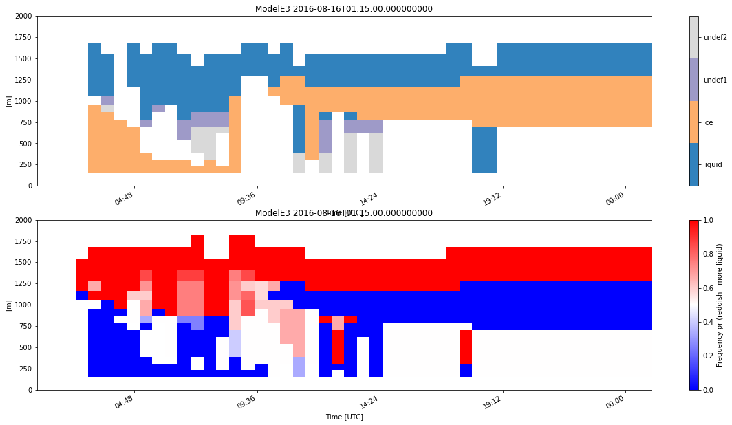
The following command will generate and process 8 subcolumns per time period of simulated HSRL data using the default radiation approach and classify the simulator output.
[5]:
my_model = emc2.simulator.main.make_simulated_data(my_model, HSRL, 8, do_classify=True, convert_zeros_to_nan=True)
## Creating subcolumns...
Now performing parallel stratiform hydrometeor allocation in subcolumns
Fully overcast cl & ci in 276 voxels
Done! total processing time = 4.77s
Now performing parallel strat precipitation allocation in subcolumns
Fully overcast pl & pi in 385 voxels
Done! total processing time = 7.19s
Now performing parallel conv precipitation allocation in subcolumns
Fully overcast pl & pi in 0 voxels
Done! total processing time = 7.37s
Generating lidar moments...
Generating stratiform lidar variables using radiation logic
Done! total processing time = 0.49s
Generating convective lidar variables using radiation logic
Done! total processing time = 0.52s
[6]:
my_model.ds
[6]:
<xarray.Dataset>
Dimensions:                     (time: 48, p: 110, subcolumn: 8)
Coordinates:
  * time                        (time) datetime64[ns] 2016-08-16T01:15:00 ......
  * p                           (p) float32 979.0 969.0 959.0 ... 0.0075 0.0035
  * subcolumn                   (subcolumn) int64 0 1 2 3 4 5 6 7
    lon                         float32 166.7
    lat                         float32 -77.85
Data variables: (12/170)
    axyp                        float32 dask.array<chunksize=(), meta=np.ndarray>
    prsurf                      (time) float32 dask.array<chunksize=(48,), meta=np.ndarray>
    gtempr                      (time) float32 dask.array<chunksize=(48,), meta=np.ndarray>
    shflx                       (time) float32 dask.array<chunksize=(48,), meta=np.ndarray>
    lhflx                       (time) float32 dask.array<chunksize=(48,), meta=np.ndarray>
    ustar                       (time) float32 dask.array<chunksize=(48,), meta=np.ndarray>
    ...                          ...
    strat_phase_mask_HSRL       (subcolumn, time, p) float64 nan nan ... nan nan
    conv_phase_mask_HSRL        (subcolumn, time, p) float64 nan nan ... nan nan
    phase_mask_HSRL_all_hyd     (subcolumn, time, p) float64 nan nan ... nan nan
    conv_COSP_phase_mask        (subcolumn, time, p) float64 nan nan ... nan nan
    strat_COSP_phase_mask       (subcolumn, time, p) float64 nan nan ... nan nan
    COSP_phase_mask_all_hyd     (subcolumn, time, p) float64 nan nan ... nan nan
Attributes:
    xlabel:               SCM_AWARE_788 SCM_AWARE (AWARE case using the Singl...
    _file_dates:          ['20160816']
    _file_times:          ['011500']
    _datastream:          act_datastream
_arm_standards_flag: 0- time: 48
- p: 110
- subcolumn: 8
- time(time)datetime64[ns]2016-08-16T01:15:00 ... 2016-08-...
array(['2016-08-16T01:15:00.000000000', '2016-08-16T01:45:00.000000000', '2016-08-16T02:15:00.000000000', '2016-08-16T02:45:00.000000000', '2016-08-16T03:15:00.000000000', '2016-08-16T03:45:00.000000000', '2016-08-16T04:15:00.000000000', '2016-08-16T04:45:00.000000000', '2016-08-16T05:15:00.000000000', '2016-08-16T05:45:00.000000000', '2016-08-16T06:15:00.000000000', '2016-08-16T06:45:00.000000000', '2016-08-16T07:15:00.000000000', '2016-08-16T07:45:00.000000000', '2016-08-16T08:15:00.000000000', '2016-08-16T08:45:00.000000000', '2016-08-16T09:15:00.000000000', '2016-08-16T09:45:00.000000000', '2016-08-16T10:15:00.000000000', '2016-08-16T10:45:00.000000000', '2016-08-16T11:15:00.000000000', '2016-08-16T11:45:00.000000000', '2016-08-16T12:15:00.000000000', '2016-08-16T12:45:00.000000000', '2016-08-16T13:15:00.000000000', '2016-08-16T13:45:00.000000000', '2016-08-16T14:15:00.000000000', '2016-08-16T14:45:00.000000000', '2016-08-16T15:15:00.000000000', '2016-08-16T15:45:00.000000000', '2016-08-16T16:15:00.000000000', '2016-08-16T16:45:00.000000000', '2016-08-16T17:15:00.000000000', '2016-08-16T17:45:00.000000000', '2016-08-16T18:15:00.000000000', '2016-08-16T18:45:00.000000000', '2016-08-16T19:15:00.000000000', '2016-08-16T19:45:00.000000000', '2016-08-16T20:15:00.000000000', '2016-08-16T20:45:00.000000000', '2016-08-16T21:15:00.000000000', '2016-08-16T21:45:00.000000000', '2016-08-16T22:15:00.000000000', '2016-08-16T22:45:00.000000000', '2016-08-16T23:15:00.000000000', '2016-08-16T23:45:00.000000000', '2016-08-17T00:15:00.000000000', '2016-08-17T00:45:00.000000000'], dtype='datetime64[ns]') - p(p)float32979.0 969.0 959.0 ... 0.0075 0.0035
array([9.79000e+02, 9.69000e+02, 9.59000e+02, 9.49000e+02, 9.39000e+02, 9.29000e+02, 9.19000e+02, 9.09000e+02, 8.99000e+02, 8.88500e+02, 8.77000e+02, 8.64500e+02, 8.51000e+02, 8.36500e+02, 8.21500e+02, 8.06500e+02, 7.91500e+02, 7.76500e+02, 7.61500e+02, 7.46500e+02, 7.31500e+02, 7.16500e+02, 7.01000e+02, 6.84500e+02, 6.67000e+02, 6.48500e+02, 6.29000e+02, 6.08500e+02, 5.87000e+02, 5.65250e+02, 5.44000e+02, 5.23250e+02, 5.03000e+02, 4.83250e+02, 4.64000e+02, 4.45250e+02, 4.27000e+02, 4.09250e+02, 3.92000e+02, 3.75250e+02, 3.59000e+02, 3.43250e+02, 3.28000e+02, 3.13250e+02, 2.99000e+02, 2.85250e+02, 2.72000e+02, 2.59250e+02, 2.47000e+02, 2.35250e+02, 2.24000e+02, 2.13250e+02, 2.03000e+02, 1.93000e+02, 1.83000e+02, 1.73000e+02, 1.63000e+02, 1.53165e+02, 1.43665e+02, 1.34500e+02, 1.25665e+02, 1.17165e+02, 1.09000e+02, 1.01165e+02, 9.36650e+01, 8.65000e+01, 7.96650e+01, 7.31650e+01, 6.70000e+01, 6.11650e+01, 5.56650e+01, 5.05000e+01, 4.56650e+01, 4.11650e+01, 3.70000e+01, 3.31650e+01, 2.96650e+01, 2.65000e+01, 2.36000e+01, 2.09000e+01, 1.84000e+01, 1.61000e+01, 1.40000e+01, 1.21000e+01, 1.04000e+01, 8.90000e+00, 7.60000e+00, 6.50000e+00, 5.55000e+00, 4.70800e+00, 3.95100e+00, 3.32600e+00, 2.80650e+00, 2.36250e+00, 1.99400e+00, 1.66850e+00, 1.39450e+00, 1.14700e+00, 9.32000e-01, 7.41000e-01, 5.63000e-01, 3.96000e-01, 2.47000e-01, 1.39000e-01, 7.80000e-02, 4.40000e-02, 2.50000e-02, 1.40000e-02, 7.50000e-03, 3.50000e-03], dtype=float32) - subcolumn(subcolumn)int640 1 2 3 4 5 6 7
array([0, 1, 2, 3, 4, 5, 6, 7])
- lon()float32166.7
- units :
- degrees_east
array(166.72, dtype=float32)
- lat()float32-77.85
- units :
- degrees_north
array(-77.85, dtype=float32)
- axyp()float32dask.array<chunksize=(), meta=np.ndarray>
- units :
- m^2
- long_name :
- gridcell area
Array Chunk Bytes 4 B 4.0 B Shape () () Count 3 Tasks 1 Chunks Type float32 numpy.ndarray - prsurf(time)float32dask.array<chunksize=(48,), meta=np.ndarray>
- units :
- hPa (mb)
- long_name :
- SURFACE PRESSURE
- mip_name :
- ps
- mip_units :
- Pa
Array Chunk Bytes 192 B 192 B Shape (48,) (48,) Count 3 Tasks 1 Chunks Type float32 numpy.ndarray - gtempr(time)float32dask.array<chunksize=(48,), meta=np.ndarray>
- units :
- K
- long_name :
- SKIN RADIATIVE TEMPERATURE
- mip_name :
- tr
Array Chunk Bytes 192 B 192 B Shape (48,) (48,) Count 3 Tasks 1 Chunks Type float32 numpy.ndarray - shflx(time)float32dask.array<chunksize=(48,), meta=np.ndarray>
- units :
- W/m^2
- long_name :
- SENSIBLE HEAT FLUX
- mip_name :
- hfss
- mip_units :
- W m-2
Array Chunk Bytes 192 B 192 B Shape (48,) (48,) Count 3 Tasks 1 Chunks Type float32 numpy.ndarray - lhflx(time)float32dask.array<chunksize=(48,), meta=np.ndarray>
- units :
- W/m^2
- long_name :
- LATENT HEAT FLUX
- mip_name :
- hfls
- mip_units :
- W m-2
Array Chunk Bytes 192 B 192 B Shape (48,) (48,) Count 3 Tasks 1 Chunks Type float32 numpy.ndarray - ustar(time)float32dask.array<chunksize=(48,), meta=np.ndarray>
- units :
- m/s
- long_name :
- FRICTION VELOCITY
Array Chunk Bytes 192 B 192 B Shape (48,) (48,) Count 3 Tasks 1 Chunks Type float32 numpy.ndarray - pblht(time)float32dask.array<chunksize=(48,), meta=np.ndarray>
- units :
- m
- long_name :
- PBL height
- mip_name :
- bldep
Array Chunk Bytes 192 B 192 B Shape (48,) (48,) Count 3 Tasks 1 Chunks Type float32 numpy.ndarray - pwv(time)float32dask.array<chunksize=(48,), meta=np.ndarray>
- units :
- kg/m^2
- long_name :
- precipitable water vapor
- mip_name :
- prw
- mip_units :
- kg m-2
Array Chunk Bytes 192 B 192 B Shape (48,) (48,) Count 3 Tasks 1 Chunks Type float32 numpy.ndarray - pblht_bp(time)float32dask.array<chunksize=(48,), meta=np.ndarray>
- units :
- m
- long_name :
- PBL height per lowest mixed layer
Array Chunk Bytes 192 B 192 B Shape (48,) (48,) Count 3 Tasks 1 Chunks Type float32 numpy.ndarray - u(time, p)float320.0 0.001123 ... 0.1097 0.1097
- long_name :
- Atmospheric optical depth
- units :
- 1
array([[0. , 0.00112319, 0.00224623, ..., 0.10968336, 0.10968336, 0.10968336], [0. , 0.00112293, 0.00224604, ..., 0.10969058, 0.10969058, 0.10969058], [0. , 0.00112301, 0.00224589, ..., 0.10969265, 0.10969265, 0.10969265], ..., [0. , 0.00112287, 0.00224563, ..., 0.1096677 , 0.1096677 , 0.1096677 ], [0. , 0.00112311, 0.00224616, ..., 0.10966126, 0.10966126, 0.10966126], [0. , 0.00112334, 0.0022467 , ..., 0.10967822, 0.10967822, 0.10967822]], dtype=float32) - v(time, p)float32dask.array<chunksize=(48, 110), meta=np.ndarray>
- units :
- m/s
- long_name :
- north-south velocity
- mip_name :
- va
- mip_units :
- m s-1
Array Chunk Bytes 20.62 kiB 20.62 kiB Shape (48, 110) (48, 110) Count 3 Tasks 1 Chunks Type float32 numpy.ndarray - t(time, p)float32dask.array<chunksize=(48, 110), meta=np.ndarray>
- units :
- K
- long_name :
- temperature
- mip_name :
- ta
Array Chunk Bytes 20.62 kiB 20.62 kiB Shape (48, 110) (48, 110) Count 3 Tasks 1 Chunks Type float32 numpy.ndarray - th(time, p)float32dask.array<chunksize=(48, 110), meta=np.ndarray>
- units :
- K
- long_name :
- potential temperature
Array Chunk Bytes 20.62 kiB 20.62 kiB Shape (48, 110) (48, 110) Count 3 Tasks 1 Chunks Type float32 numpy.ndarray - q(time, p)float32dask.array<chunksize=(48, 110), meta=np.ndarray>
- units :
- kg/kg
- long_name :
- specific humidity
- mip_name :
- hus
- mip_units :
- 1
Array Chunk Bytes 20.62 kiB 20.62 kiB Shape (48, 110) (48, 110) Count 3 Tasks 1 Chunks Type float32 numpy.ndarray - rhw(time, p)float32dask.array<chunksize=(48, 110), meta=np.ndarray>
- units :
- %
- long_name :
- relative humidity (water)
Array Chunk Bytes 20.62 kiB 20.62 kiB Shape (48, 110) (48, 110) Count 3 Tasks 1 Chunks Type float32 numpy.ndarray - z(time, p)float32dask.array<chunksize=(48, 110), meta=np.ndarray>
- units :
- m
- long_name :
- layer altitude (above MSL)
- mip_name :
- zg
Array Chunk Bytes 20.62 kiB 20.62 kiB Shape (48, 110) (48, 110) Count 3 Tasks 1 Chunks Type float32 numpy.ndarray - p_3d(time, p)float32dask.array<chunksize=(48, 110), meta=np.ndarray>
- units :
- hPa
- long_name :
- pressure on model levels
- mip_name :
- pfull
- mip_units :
- Pa
Array Chunk Bytes 20.62 kiB 20.62 kiB Shape (48, 110) (48, 110) Count 3 Tasks 1 Chunks Type float32 numpy.ndarray - olr(time)float32dask.array<chunksize=(48,), meta=np.ndarray>
- units :
- W/m^2
- long_name :
- OUTGOING LW RADIATION at TOA (in RADIA)
- mip_name :
- rlut
- mip_units :
- W m-2
Array Chunk Bytes 192 B 192 B Shape (48,) (48,) Count 3 Tasks 1 Chunks Type float32 numpy.ndarray - olrcs(time)float32dask.array<chunksize=(48,), meta=np.ndarray>
- units :
- W/m^2
- long_name :
- OUTGOING LW RADIATION at TOA, CLEAR-SKY
- mip_name :
- rlutcs
- mip_units :
- W m-2
Array Chunk Bytes 192 B 192 B Shape (48,) (48,) Count 3 Tasks 1 Chunks Type float32 numpy.ndarray - lwds(time)float32dask.array<chunksize=(48,), meta=np.ndarray>
- units :
- W/m^2
- long_name :
- LONGWAVE DOWNWARD FLUX at SURFACE
- mip_name :
- rlds
- mip_units :
- W m-2
Array Chunk Bytes 192 B 192 B Shape (48,) (48,) Count 3 Tasks 1 Chunks Type float32 numpy.ndarray - lwdscs(time)float32dask.array<chunksize=(48,), meta=np.ndarray>
- units :
- W/m^2
- long_name :
- LONGWAVE DOWNWARD FLUX at SURFACE, CLEAR-SKY
- mip_name :
- rldscs
- mip_units :
- W m-2
Array Chunk Bytes 192 B 192 B Shape (48,) (48,) Count 3 Tasks 1 Chunks Type float32 numpy.ndarray - lwus(time)float32dask.array<chunksize=(48,), meta=np.ndarray>
- units :
- W/m^2
- long_name :
- LONGWAVE UPWARD FLUX at SURFACE
- mip_name :
- rlus
- mip_units :
- W m-2
Array Chunk Bytes 192 B 192 B Shape (48,) (48,) Count 3 Tasks 1 Chunks Type float32 numpy.ndarray - swds(time)float32dask.array<chunksize=(48,), meta=np.ndarray>
- units :
- W/m^2
- long_name :
- SOLAR DOWNWARD FLUX at SURFACE
- mip_name :
- rsds
- mip_units :
- W m-2
Array Chunk Bytes 192 B 192 B Shape (48,) (48,) Count 3 Tasks 1 Chunks Type float32 numpy.ndarray - swus(time)float32dask.array<chunksize=(48,), meta=np.ndarray>
- units :
- W/m^2
- long_name :
- SOLAR UPWARD FLUX at SURFACE
- mip_name :
- rsus
- mip_units :
- W m-2
Array Chunk Bytes 192 B 192 B Shape (48,) (48,) Count 3 Tasks 1 Chunks Type float32 numpy.ndarray - swnscs(time)float32dask.array<chunksize=(48,), meta=np.ndarray>
- units :
- W/m^2
- long_name :
- Clear-sky solar net flux at surface
Array Chunk Bytes 192 B 192 B Shape (48,) (48,) Count 3 Tasks 1 Chunks Type float32 numpy.ndarray - swdf(time)float32dask.array<chunksize=(48,), meta=np.ndarray>
- units :
- W/m^2
- long_name :
- SOLAR DOWNWARD DIFFUSE FLUX at SURFACE
- mip_name :
- rsdsdiff
- mip_units :
- W m-2
Array Chunk Bytes 192 B 192 B Shape (48,) (48,) Count 3 Tasks 1 Chunks Type float32 numpy.ndarray - lwdp(time, p)float32dask.array<chunksize=(48, 110), meta=np.ndarray>
- units :
- W/m^2
- long_name :
- Longwave downward flux profile
- mip_name :
- rld
- mip_units :
- W m-2
Array Chunk Bytes 20.62 kiB 20.62 kiB Shape (48, 110) (48, 110) Count 3 Tasks 1 Chunks Type float32 numpy.ndarray - swdp(time, p)float32dask.array<chunksize=(48, 110), meta=np.ndarray>
- units :
- W/m^2
- long_name :
- Shortwave downward flux profile
- mip_name :
- rsd
- mip_units :
- W m-2
Array Chunk Bytes 20.62 kiB 20.62 kiB Shape (48, 110) (48, 110) Count 3 Tasks 1 Chunks Type float32 numpy.ndarray - dth_sw(time, p)float32dask.array<chunksize=(48, 110), meta=np.ndarray>
- units :
- K/day
- long_name :
- theta tendency from shortwave radiative heating
Array Chunk Bytes 20.62 kiB 20.62 kiB Shape (48, 110) (48, 110) Count 3 Tasks 1 Chunks Type float32 numpy.ndarray - dth_lw(time, p)float32dask.array<chunksize=(48, 110), meta=np.ndarray>
- units :
- K/day
- long_name :
- theta tendency from longwave radiative heating
Array Chunk Bytes 20.62 kiB 20.62 kiB Shape (48, 110) (48, 110) Count 3 Tasks 1 Chunks Type float32 numpy.ndarray - dth_rad(time, p)float32dask.array<chunksize=(48, 110), meta=np.ndarray>
- units :
- K/day
- long_name :
- theta tendency from radiative heating
Array Chunk Bytes 20.62 kiB 20.62 kiB Shape (48, 110) (48, 110) Count 3 Tasks 1 Chunks Type float32 numpy.ndarray - lwup(time, p)float32dask.array<chunksize=(48, 110), meta=np.ndarray>
- units :
- W/m^2
- long_name :
- Longwave upward flux profile
- mip_name :
- rlu
- mip_units :
- W m-2
Array Chunk Bytes 20.62 kiB 20.62 kiB Shape (48, 110) (48, 110) Count 3 Tasks 1 Chunks Type float32 numpy.ndarray - swup(time, p)float32dask.array<chunksize=(48, 110), meta=np.ndarray>
- units :
- W/m^2
- long_name :
- Shortwave upward flux profile
- mip_name :
- rsu
- mip_units :
- W m-2
Array Chunk Bytes 20.62 kiB 20.62 kiB Shape (48, 110) (48, 110) Count 3 Tasks 1 Chunks Type float32 numpy.ndarray - dq_turb(time, p)float32dask.array<chunksize=(48, 110), meta=np.ndarray>
- units :
- kg/kg/day
- long_name :
- moisture tendency from surface fluxes and turbulence
- mip_name :
- tnhuspbl
- mip_units :
- s-1
Array Chunk Bytes 20.62 kiB 20.62 kiB Shape (48, 110) (48, 110) Count 3 Tasks 1 Chunks Type float32 numpy.ndarray - dth_turb(time, p)float32dask.array<chunksize=(48, 110), meta=np.ndarray>
- units :
- K/day
- long_name :
- theta tendency from surface fluxes and turbulence
Array Chunk Bytes 20.62 kiB 20.62 kiB Shape (48, 110) (48, 110) Count 3 Tasks 1 Chunks Type float32 numpy.ndarray - e_turb(time, p)float32dask.array<chunksize=(48, 110), meta=np.ndarray>
- units :
- m2/s2
- long_name :
- atmospheric turbulent kinetic energy
Array Chunk Bytes 20.62 kiB 20.62 kiB Shape (48, 110) (48, 110) Count 3 Tasks 1 Chunks Type float32 numpy.ndarray - km_turb(time, p)float32dask.array<chunksize=(48, 110), meta=np.ndarray>
- units :
- m2/s
- long_name :
- turbulent diffusivity for momentum
- mip_name :
- evu
- mip_units :
- m2 s-1
Array Chunk Bytes 20.62 kiB 20.62 kiB Shape (48, 110) (48, 110) Count 3 Tasks 1 Chunks Type float32 numpy.ndarray - kh_turb(time, p)float32dask.array<chunksize=(48, 110), meta=np.ndarray>
- units :
- m2/s
- long_name :
- turbulent diffusivity for heat
- mip_name :
- edt
- mip_units :
- m2 s-1
Array Chunk Bytes 20.62 kiB 20.62 kiB Shape (48, 110) (48, 110) Count 3 Tasks 1 Chunks Type float32 numpy.ndarray - ri_turb(time, p)float32dask.array<chunksize=(48, 110), meta=np.ndarray>
- units :
- 1
- long_name :
- turbulent Richardson number
Array Chunk Bytes 20.62 kiB 20.62 kiB Shape (48, 110) (48, 110) Count 3 Tasks 1 Chunks Type float32 numpy.ndarray - len_turb(time, p)float32dask.array<chunksize=(48, 110), meta=np.ndarray>
- units :
- m
- long_name :
- turbulent length scale
Array Chunk Bytes 20.62 kiB 20.62 kiB Shape (48, 110) (48, 110) Count 3 Tasks 1 Chunks Type float32 numpy.ndarray - prec(time)float32dask.array<chunksize=(48,), meta=np.ndarray>
- units :
- mm/d
- long_name :
- Surface Precipitation Rate
- mip_name :
- pr
- mip_units :
- kg m-2 s-1
Array Chunk Bytes 192 B 192 B Shape (48,) (48,) Count 3 Tasks 1 Chunks Type float32 numpy.ndarray - mcp(time)float32dask.array<chunksize=(48,), meta=np.ndarray>
- units :
- mm/d
- long_name :
- Convective Surface Precipitation Rate
- mip_name :
- prc
- mip_units :
- kg m-2 s-1
Array Chunk Bytes 192 B 192 B Shape (48,) (48,) Count 3 Tasks 1 Chunks Type float32 numpy.ndarray - ssp(time)float32dask.array<chunksize=(48,), meta=np.ndarray>
- units :
- mm/d
- long_name :
- Stratiform Surface Precipitation Rate
Array Chunk Bytes 192 B 192 B Shape (48,) (48,) Count 3 Tasks 1 Chunks Type float32 numpy.ndarray - cldmc_2d(time)float32dask.array<chunksize=(48,), meta=np.ndarray>
- units :
- %
- long_name :
- Convective Cloud Cover
- mip_name :
- cltc
Array Chunk Bytes 192 B 192 B Shape (48,) (48,) Count 3 Tasks 1 Chunks Type float32 numpy.ndarray - cldss_2d(time)float32dask.array<chunksize=(48,), meta=np.ndarray>
- units :
- %
- long_name :
- Stratiform Cloud Cover
Array Chunk Bytes 192 B 192 B Shape (48,) (48,) Count 3 Tasks 1 Chunks Type float32 numpy.ndarray - cldtot_2d(time)float32dask.array<chunksize=(48,), meta=np.ndarray>
- units :
- %
- long_name :
- Total Cloud Cover
Array Chunk Bytes 192 B 192 B Shape (48,) (48,) Count 3 Tasks 1 Chunks Type float32 numpy.ndarray - lwp(time)float32dask.array<chunksize=(48,), meta=np.ndarray>
- units :
- g/m^2
- long_name :
- Liquid Water Path
Array Chunk Bytes 192 B 192 B Shape (48,) (48,) Count 3 Tasks 1 Chunks Type float32 numpy.ndarray - iwp(time)float32dask.array<chunksize=(48,), meta=np.ndarray>
- units :
- g/m^2
- long_name :
- Ice Water Path
- mip_name :
- clivi
- mip_units :
- kg m-2
Array Chunk Bytes 192 B 192 B Shape (48,) (48,) Count 3 Tasks 1 Chunks Type float32 numpy.ndarray - cLWPss(time)float32dask.array<chunksize=(48,), meta=np.ndarray>
- units :
- g/m^2
- long_name :
- Stratiform Cloud Liquid Water Path
Array Chunk Bytes 192 B 192 B Shape (48,) (48,) Count 3 Tasks 1 Chunks Type float32 numpy.ndarray - pLWPss(time)float32dask.array<chunksize=(48,), meta=np.ndarray>
- units :
- g/m^2
- long_name :
- Stratiform Rain Liquid Water Path
Array Chunk Bytes 192 B 192 B Shape (48,) (48,) Count 3 Tasks 1 Chunks Type float32 numpy.ndarray - cIWPss(time)float32dask.array<chunksize=(48,), meta=np.ndarray>
- units :
- g/m^2
- long_name :
- Stratiform Cloud Ice Water Path
Array Chunk Bytes 192 B 192 B Shape (48,) (48,) Count 3 Tasks 1 Chunks Type float32 numpy.ndarray - pIWPss(time)float32dask.array<chunksize=(48,), meta=np.ndarray>
- units :
- g/m^2
- long_name :
- Stratiform Snow Ice Water Path
Array Chunk Bytes 192 B 192 B Shape (48,) (48,) Count 3 Tasks 1 Chunks Type float32 numpy.ndarray - qcl(time, p)float32dask.array<chunksize=(48, 110), meta=np.ndarray>
- units :
- kg/kg
- long_name :
- Stratiform Cloud Water
Array Chunk Bytes 20.62 kiB 20.62 kiB Shape (48, 110) (48, 110) Count 3 Tasks 1 Chunks Type float32 numpy.ndarray - qci(time, p)float32dask.array<chunksize=(48, 110), meta=np.ndarray>
- units :
- kg/kg
- long_name :
- Stratiform Cloud Ice
Array Chunk Bytes 20.62 kiB 20.62 kiB Shape (48, 110) (48, 110) Count 3 Tasks 1 Chunks Type float32 numpy.ndarray - nclic(time, p)float32dask.array<chunksize=(48, 110), meta=np.ndarray>
- units :
- cm-3
- long_name :
- Stratiform Cloud Droplets In-cloud
Array Chunk Bytes 20.62 kiB 20.62 kiB Shape (48, 110) (48, 110) Count 3 Tasks 1 Chunks Type float32 numpy.ndarray - nciic(time, p)float32dask.array<chunksize=(48, 110), meta=np.ndarray>
- units :
- cm-3
- long_name :
- Stratiform Cloud Ice Crystals In-cloud
Array Chunk Bytes 20.62 kiB 20.62 kiB Shape (48, 110) (48, 110) Count 3 Tasks 1 Chunks Type float32 numpy.ndarray - cldss(time, p)float32dask.array<chunksize=(48, 110), meta=np.ndarray>
- units :
- -
- long_name :
- Stratiform Cloud Fraction (no precip)
Array Chunk Bytes 20.62 kiB 20.62 kiB Shape (48, 110) (48, 110) Count 3 Tasks 1 Chunks Type float32 numpy.ndarray - cldsscl(time, p)float32dask.array<chunksize=(48, 110), meta=np.ndarray>
- units :
- -
- long_name :
- Stratiform Water Cloud Fraction
Array Chunk Bytes 20.62 kiB 20.62 kiB Shape (48, 110) (48, 110) Count 3 Tasks 1 Chunks Type float32 numpy.ndarray - cldssci(time, p)float32dask.array<chunksize=(48, 110), meta=np.ndarray>
- units :
- -
- long_name :
- Stratiform Ice Cloud Fraction
Array Chunk Bytes 20.62 kiB 20.62 kiB Shape (48, 110) (48, 110) Count 3 Tasks 1 Chunks Type float32 numpy.ndarray - cldmc(time, p)float32dask.array<chunksize=(48, 110), meta=np.ndarray>
- units :
- -
- long_name :
- Convective Cloud Fraction (no precip)
Array Chunk Bytes 20.62 kiB 20.62 kiB Shape (48, 110) (48, 110) Count 3 Tasks 1 Chunks Type float32 numpy.ndarray - qpl(time, p)float32dask.array<chunksize=(48, 110), meta=np.ndarray>
- units :
- kg/kg
- long_name :
- Stratiform Rainwater
Array Chunk Bytes 20.62 kiB 20.62 kiB Shape (48, 110) (48, 110) Count 3 Tasks 1 Chunks Type float32 numpy.ndarray - qpi(time, p)float32dask.array<chunksize=(48, 110), meta=np.ndarray>
- units :
- kg/kg
- long_name :
- Stratiform Snow
Array Chunk Bytes 20.62 kiB 20.62 kiB Shape (48, 110) (48, 110) Count 3 Tasks 1 Chunks Type float32 numpy.ndarray - dtau_ss(time, p)float32dask.array<chunksize=(48, 110), meta=np.ndarray>
- units :
- -
- long_name :
- Stratiform Cloud Optical Depth
- mip_name :
- dtaus
- mip_units :
- 1
Array Chunk Bytes 20.62 kiB 20.62 kiB Shape (48, 110) (48, 110) Count 3 Tasks 1 Chunks Type float32 numpy.ndarray - dtau_mc(time, p)float32dask.array<chunksize=(48, 110), meta=np.ndarray>
- units :
- -
- long_name :
- Convective Cloud Optical Depth
- mip_name :
- dtauc
- mip_units :
- 1
Array Chunk Bytes 20.62 kiB 20.62 kiB Shape (48, 110) (48, 110) Count 3 Tasks 1 Chunks Type float32 numpy.ndarray - dq_mc(time, p)float32dask.array<chunksize=(48, 110), meta=np.ndarray>
- units :
- kg/kg/day
- long_name :
- Moisture Tendency from Moist Convection
- mip_name :
- tnhusc
- mip_units :
- s-1
Array Chunk Bytes 20.62 kiB 20.62 kiB Shape (48, 110) (48, 110) Count 3 Tasks 1 Chunks Type float32 numpy.ndarray - dth_mc(time, p)float32dask.array<chunksize=(48, 110), meta=np.ndarray>
- units :
- K/day
- long_name :
- Theta Tendency from Moist Convection
Array Chunk Bytes 20.62 kiB 20.62 kiB Shape (48, 110) (48, 110) Count 3 Tasks 1 Chunks Type float32 numpy.ndarray - dq_ss(time, p)float32dask.array<chunksize=(48, 110), meta=np.ndarray>
- units :
- kg/kg/day
- long_name :
- Moisture Tendency from Stratiform Cloud
- mip_name :
- tnhusscp
- mip_units :
- s-1
Array Chunk Bytes 20.62 kiB 20.62 kiB Shape (48, 110) (48, 110) Count 3 Tasks 1 Chunks Type float32 numpy.ndarray - dth_ss(time, p)float32dask.array<chunksize=(48, 110), meta=np.ndarray>
- units :
- K/day
- long_name :
- Theta Tendency from Stratiform Cloud
Array Chunk Bytes 20.62 kiB 20.62 kiB Shape (48, 110) (48, 110) Count 3 Tasks 1 Chunks Type float32 numpy.ndarray - cldssr(time, p)float32dask.array<chunksize=(48, 110), meta=np.ndarray>
- units :
- -
- long_name :
- Stratiform Cloud Fraction (includes precip seen by radiation)
- mip_name :
- cls
- mip_units :
- %
Array Chunk Bytes 20.62 kiB 20.62 kiB Shape (48, 110) (48, 110) Count 3 Tasks 1 Chunks Type float32 numpy.ndarray - cldmcr(time, p)float32dask.array<chunksize=(48, 110), meta=np.ndarray>
- units :
- -
- long_name :
- Convective Cloud Fraction (includes precip seen by radiation)
- mip_name :
- clc
- mip_units :
- %
Array Chunk Bytes 20.62 kiB 20.62 kiB Shape (48, 110) (48, 110) Count 3 Tasks 1 Chunks Type float32 numpy.ndarray - QCLmc(time, p)float32dask.array<chunksize=(48, 110), meta=np.ndarray>
- units :
- kg/kg
- long_name :
- Convective Cloud Water
Array Chunk Bytes 20.62 kiB 20.62 kiB Shape (48, 110) (48, 110) Count 3 Tasks 1 Chunks Type float32 numpy.ndarray - QCImc(time, p)float32dask.array<chunksize=(48, 110), meta=np.ndarray>
- units :
- kg/kg
- long_name :
- Convective Cloud Ice
Array Chunk Bytes 20.62 kiB 20.62 kiB Shape (48, 110) (48, 110) Count 3 Tasks 1 Chunks Type float32 numpy.ndarray - QPLmc(time, p)float32dask.array<chunksize=(48, 110), meta=np.ndarray>
- units :
- kg/kg
- long_name :
- Convective Rainwater
Array Chunk Bytes 20.62 kiB 20.62 kiB Shape (48, 110) (48, 110) Count 3 Tasks 1 Chunks Type float32 numpy.ndarray - QPImc(time, p)float32dask.array<chunksize=(48, 110), meta=np.ndarray>
- units :
- kg/kg
- long_name :
- Convective Snow
Array Chunk Bytes 20.62 kiB 20.62 kiB Shape (48, 110) (48, 110) Count 3 Tasks 1 Chunks Type float32 numpy.ndarray - re_mccl(time, p)float32dask.array<chunksize=(48, 110), meta=np.ndarray>
- units :
- micron
- long_name :
- Convective Cloud Droplet Effective Radius
- mip_name :
- reffclwc
- mip_units :
- m
Array Chunk Bytes 20.62 kiB 20.62 kiB Shape (48, 110) (48, 110) Count 3 Tasks 1 Chunks Type float32 numpy.ndarray - re_mcci(time, p)float32dask.array<chunksize=(48, 110), meta=np.ndarray>
- units :
- micron
- long_name :
- Convective Cloud Ice Effective Radius
- mip_name :
- reffclic
- mip_units :
- m
Array Chunk Bytes 20.62 kiB 20.62 kiB Shape (48, 110) (48, 110) Count 3 Tasks 1 Chunks Type float32 numpy.ndarray - re_mcpl(time, p)float32dask.array<chunksize=(48, 110), meta=np.ndarray>
- units :
- micron
- long_name :
- Convective Raindrop Effective Radius
- mip_name :
- reffrainc
- mip_units :
- m
Array Chunk Bytes 20.62 kiB 20.62 kiB Shape (48, 110) (48, 110) Count 3 Tasks 1 Chunks Type float32 numpy.ndarray - re_mcpi(time, p)float32dask.array<chunksize=(48, 110), meta=np.ndarray>
- units :
- micron
- long_name :
- Convective Precipitating Ice Effective Radius
- mip_name :
- reffsnowc
- mip_units :
- m
Array Chunk Bytes 20.62 kiB 20.62 kiB Shape (48, 110) (48, 110) Count 3 Tasks 1 Chunks Type float32 numpy.ndarray - ncl(time, p)float32dask.array<chunksize=(48, 110), meta=np.ndarray>
- units :
- cm-3
- long_name :
- Stratiform Cloud Droplets
Array Chunk Bytes 20.62 kiB 20.62 kiB Shape (48, 110) (48, 110) Count 3 Tasks 1 Chunks Type float32 numpy.ndarray - npl(time, p)float32dask.array<chunksize=(48, 110), meta=np.ndarray>
- units :
- cm-3
- long_name :
- Stratiform Raindrops
Array Chunk Bytes 20.62 kiB 20.62 kiB Shape (48, 110) (48, 110) Count 3 Tasks 1 Chunks Type float32 numpy.ndarray - nci(time, p)float32dask.array<chunksize=(48, 110), meta=np.ndarray>
- units :
- cm-3
- long_name :
- Stratiform Cloud Ice Crystals
Array Chunk Bytes 20.62 kiB 20.62 kiB Shape (48, 110) (48, 110) Count 3 Tasks 1 Chunks Type float32 numpy.ndarray - npi(time, p)float32dask.array<chunksize=(48, 110), meta=np.ndarray>
- units :
- cm-3
- long_name :
- Stratiform Snow Crystals
Array Chunk Bytes 20.62 kiB 20.62 kiB Shape (48, 110) (48, 110) Count 3 Tasks 1 Chunks Type float32 numpy.ndarray - cldsspl(time, p)float32dask.array<chunksize=(48, 110), meta=np.ndarray>
- units :
- -
- long_name :
- Stratiform Rain Fraction
Array Chunk Bytes 20.62 kiB 20.62 kiB Shape (48, 110) (48, 110) Count 3 Tasks 1 Chunks Type float32 numpy.ndarray - cldsspi(time, p)float32dask.array<chunksize=(48, 110), meta=np.ndarray>
- units :
- -
- long_name :
- Stratiform Snow Fraction
Array Chunk Bytes 20.62 kiB 20.62 kiB Shape (48, 110) (48, 110) Count 3 Tasks 1 Chunks Type float32 numpy.ndarray - cldmccl(time, p)float32dask.array<chunksize=(48, 110), meta=np.ndarray>
- units :
- -
- long_name :
- Convective Cloud Water Fraction
Array Chunk Bytes 20.62 kiB 20.62 kiB Shape (48, 110) (48, 110) Count 3 Tasks 1 Chunks Type float32 numpy.ndarray - cldmcpl(time, p)float32dask.array<chunksize=(48, 110), meta=np.ndarray>
- units :
- -
- long_name :
- Convective Rain Fraction
Array Chunk Bytes 20.62 kiB 20.62 kiB Shape (48, 110) (48, 110) Count 3 Tasks 1 Chunks Type float32 numpy.ndarray - cldmcci(time, p)float32dask.array<chunksize=(48, 110), meta=np.ndarray>
- units :
- -
- long_name :
- Convective Cloud Ice Fraction
Array Chunk Bytes 20.62 kiB 20.62 kiB Shape (48, 110) (48, 110) Count 3 Tasks 1 Chunks Type float32 numpy.ndarray - cldmcpi(time, p)float32dask.array<chunksize=(48, 110), meta=np.ndarray>
- units :
- -
- long_name :
- Convective Snow Fraction
Array Chunk Bytes 20.62 kiB 20.62 kiB Shape (48, 110) (48, 110) Count 3 Tasks 1 Chunks Type float32 numpy.ndarray - re_sscl(time, p)float32dask.array<chunksize=(48, 110), meta=np.ndarray>
- units :
- micron
- long_name :
- Stratiform Cloud Droplet Effective Radius
- mip_name :
- reffclws
- mip_units :
- m
Array Chunk Bytes 20.62 kiB 20.62 kiB Shape (48, 110) (48, 110) Count 3 Tasks 1 Chunks Type float32 numpy.ndarray - re_ssci(time, p)float32dask.array<chunksize=(48, 110), meta=np.ndarray>
- units :
- micron
- long_name :
- Stratiform Cloud Ice Effective Radius
- mip_name :
- reffclis
- mip_units :
- m
Array Chunk Bytes 20.62 kiB 20.62 kiB Shape (48, 110) (48, 110) Count 3 Tasks 1 Chunks Type float32 numpy.ndarray - re_sspl(time, p)float32dask.array<chunksize=(48, 110), meta=np.ndarray>
- units :
- micron
- long_name :
- Stratiform Raindrop Effective Radius
- mip_name :
- reffrains
- mip_units :
- m
Array Chunk Bytes 20.62 kiB 20.62 kiB Shape (48, 110) (48, 110) Count 3 Tasks 1 Chunks Type float32 numpy.ndarray - re_sspi(time, p)float32dask.array<chunksize=(48, 110), meta=np.ndarray>
- units :
- micron
- long_name :
- Stratiform Snow Effective Radius
- mip_name :
- reffsnows
- mip_units :
- m
Array Chunk Bytes 20.62 kiB 20.62 kiB Shape (48, 110) (48, 110) Count 3 Tasks 1 Chunks Type float32 numpy.ndarray - dq_ls(time, p)float32dask.array<chunksize=(48, 110), meta=np.ndarray>
- units :
- kg/kg/d
- long_name :
- moisture tendency from large-scale forcings
Array Chunk Bytes 20.62 kiB 20.62 kiB Shape (48, 110) (48, 110) Count 3 Tasks 1 Chunks Type float32 numpy.ndarray - dth_ls(time, p)float32dask.array<chunksize=(48, 110), meta=np.ndarray>
- units :
- K/d
- long_name :
- theta tendency from large-scale forcings
Array Chunk Bytes 20.62 kiB 20.62 kiB Shape (48, 110) (48, 110) Count 3 Tasks 1 Chunks Type float32 numpy.ndarray - dq_nudge(time, p)float32dask.array<chunksize=(48, 110), meta=np.ndarray>
- units :
- kg/kg/d
- long_name :
- moisture tendency from nudging
Array Chunk Bytes 20.62 kiB 20.62 kiB Shape (48, 110) (48, 110) Count 3 Tasks 1 Chunks Type float32 numpy.ndarray - dth_nudge(time, p)float32dask.array<chunksize=(48, 110), meta=np.ndarray>
- units :
- K/d
- long_name :
- theta tendency from nudging
Array Chunk Bytes 20.62 kiB 20.62 kiB Shape (48, 110) (48, 110) Count 3 Tasks 1 Chunks Type float32 numpy.ndarray - conv_frac_subcolumns_cl(subcolumn, time, p)boolFalse False False ... False False
- units :
- boolean
- long_name :
- Is there hydrometeors of type cl in each subcolumn?
- Processing method :
- Radiation logic
array([[[False, False, False, ..., False, False, False], [False, False, False, ..., False, False, False], [False, False, False, ..., False, False, False], ..., [False, False, False, ..., False, False, False], [False, False, False, ..., False, False, False], [False, False, False, ..., False, False, False]], [[False, False, False, ..., False, False, False], [False, False, False, ..., False, False, False], [False, False, False, ..., False, False, False], ..., [False, False, False, ..., False, False, False], [False, False, False, ..., False, False, False], [False, False, False, ..., False, False, False]], [[False, False, False, ..., False, False, False], [False, False, False, ..., False, False, False], [False, False, False, ..., False, False, False], ..., ... ..., [False, False, False, ..., False, False, False], [False, False, False, ..., False, False, False], [False, False, False, ..., False, False, False]], [[False, False, False, ..., False, False, False], [False, False, False, ..., False, False, False], [False, False, False, ..., False, False, False], ..., [False, False, False, ..., False, False, False], [False, False, False, ..., False, False, False], [False, False, False, ..., False, False, False]], [[False, False, False, ..., False, False, False], [False, False, False, ..., False, False, False], [False, False, False, ..., False, False, False], ..., [False, False, False, ..., False, False, False], [False, False, False, ..., False, False, False], [False, False, False, ..., False, False, False]]]) - conv_frac_subcolumns_ci(subcolumn, time, p)boolFalse False False ... False False
- units :
- boolean
- long_name :
- Is there hydrometeors of type ci in each subcolumn?
- Processing method :
- Radiation logic
array([[[False, False, False, ..., False, False, False], [False, False, False, ..., False, False, False], [False, False, False, ..., False, False, False], ..., [False, False, False, ..., False, False, False], [False, False, False, ..., False, False, False], [False, False, False, ..., False, False, False]], [[False, False, False, ..., False, False, False], [False, False, False, ..., False, False, False], [False, False, False, ..., False, False, False], ..., [False, False, False, ..., False, False, False], [False, False, False, ..., False, False, False], [False, False, False, ..., False, False, False]], [[False, False, False, ..., False, False, False], [False, False, False, ..., False, False, False], [False, False, False, ..., False, False, False], ..., ... ..., [False, False, False, ..., False, False, False], [False, False, False, ..., False, False, False], [False, False, False, ..., False, False, False]], [[False, False, False, ..., False, False, False], [False, False, False, ..., False, False, False], [False, False, False, ..., False, False, False], ..., [False, False, False, ..., False, False, False], [False, False, False, ..., False, False, False], [False, False, False, ..., False, False, False]], [[False, False, False, ..., False, False, False], [False, False, False, ..., False, False, False], [False, False, False, ..., False, False, False], ..., [False, False, False, ..., False, False, False], [False, False, False, ..., False, False, False], [False, False, False, ..., False, False, False]]]) - conv_frac_subcolumns_pl(subcolumn, time, p)boolFalse False False ... False False
- long_name :
- Liquid precipitation present? [convective]
- units :
- 0 = no, 1 = yes
- Processing method :
- Radiation logic
array([[[False, False, False, ..., False, False, False], [False, False, False, ..., False, False, False], [False, False, False, ..., False, False, False], ..., [False, False, False, ..., False, False, False], [False, False, False, ..., False, False, False], [False, False, False, ..., False, False, False]], [[False, False, False, ..., False, False, False], [False, False, False, ..., False, False, False], [False, False, False, ..., False, False, False], ..., [False, False, False, ..., False, False, False], [False, False, False, ..., False, False, False], [False, False, False, ..., False, False, False]], [[False, False, False, ..., False, False, False], [False, False, False, ..., False, False, False], [False, False, False, ..., False, False, False], ..., ... ..., [False, False, False, ..., False, False, False], [False, False, False, ..., False, False, False], [False, False, False, ..., False, False, False]], [[False, False, False, ..., False, False, False], [False, False, False, ..., False, False, False], [False, False, False, ..., False, False, False], ..., [False, False, False, ..., False, False, False], [False, False, False, ..., False, False, False], [False, False, False, ..., False, False, False]], [[False, False, False, ..., False, False, False], [False, False, False, ..., False, False, False], [False, False, False, ..., False, False, False], ..., [False, False, False, ..., False, False, False], [False, False, False, ..., False, False, False], [False, False, False, ..., False, False, False]]]) - conv_frac_subcolumns_pi(subcolumn, time, p)boolFalse False False ... False False
- long_name :
- Ice precipitation present? [convective]
- units :
- 0 = no, 1 = yes
- Processing method :
- Radiation logic
array([[[False, False, False, ..., False, False, False], [False, False, False, ..., False, False, False], [False, False, False, ..., False, False, False], ..., [False, False, False, ..., False, False, False], [False, False, False, ..., False, False, False], [False, False, False, ..., False, False, False]], [[False, False, False, ..., False, False, False], [False, False, False, ..., False, False, False], [False, False, False, ..., False, False, False], ..., [False, False, False, ..., False, False, False], [False, False, False, ..., False, False, False], [False, False, False, ..., False, False, False]], [[False, False, False, ..., False, False, False], [False, False, False, ..., False, False, False], [False, False, False, ..., False, False, False], ..., ... ..., [False, False, False, ..., False, False, False], [False, False, False, ..., False, False, False], [False, False, False, ..., False, False, False]], [[False, False, False, ..., False, False, False], [False, False, False, ..., False, False, False], [False, False, False, ..., False, False, False], ..., [False, False, False, ..., False, False, False], [False, False, False, ..., False, False, False], [False, False, False, ..., False, False, False]], [[False, False, False, ..., False, False, False], [False, False, False, ..., False, False, False], [False, False, False, ..., False, False, False], ..., [False, False, False, ..., False, False, False], [False, False, False, ..., False, False, False], [False, False, False, ..., False, False, False]]]) - strat_frac_subcolumns_cl(subcolumn, time, p)boolFalse False False ... False False
- long_name :
- Liquid cloud particles present? [stratiform]
- units :
- 0 = no, 1 = yes
- Processing method :
- Radiation logic
array([[[False, False, False, ..., False, False, False], [False, False, False, ..., False, False, False], [False, False, False, ..., False, False, False], ..., [False, False, False, ..., False, False, False], [False, False, False, ..., False, False, False], [False, False, False, ..., False, False, False]], [[False, False, False, ..., False, False, False], [False, False, False, ..., False, False, False], [False, False, False, ..., False, False, False], ..., [False, False, False, ..., False, False, False], [False, False, False, ..., False, False, False], [False, False, False, ..., False, False, False]], [[False, False, False, ..., False, False, False], [False, False, False, ..., False, False, False], [False, False, False, ..., False, False, False], ..., ... ..., [False, False, False, ..., False, False, False], [False, False, False, ..., False, False, False], [False, False, False, ..., False, False, False]], [[False, False, False, ..., False, False, False], [False, False, False, ..., False, False, False], [False, False, False, ..., False, False, False], ..., [False, False, False, ..., False, False, False], [ True, True, True, ..., False, False, False], [False, False, False, ..., False, False, False]], [[False, False, False, ..., False, False, False], [False, False, False, ..., False, False, False], [False, False, False, ..., False, False, False], ..., [ True, True, True, ..., False, False, False], [False, False, False, ..., False, False, False], [False, False, False, ..., False, False, False]]]) - strat_frac_subcolumns_ci(subcolumn, time, p)boolFalse False False ... False False
- long_name :
- Liquid cloud particles present? [stratiform]
- units :
- 0 = no, 1 = yes
- Processing method :
- Radiation logic
array([[[False, False, False, ..., False, False, False], [False, False, False, ..., False, False, False], [False, False, False, ..., False, False, False], ..., [False, False, False, ..., False, False, False], [False, False, False, ..., False, False, False], [False, False, False, ..., False, False, False]], [[False, False, False, ..., False, False, False], [False, False, False, ..., False, False, False], [False, False, False, ..., False, False, False], ..., [False, False, False, ..., False, False, False], [False, False, False, ..., False, False, False], [False, False, False, ..., False, False, False]], [[False, False, False, ..., False, False, False], [False, False, False, ..., False, False, False], [False, False, False, ..., False, False, False], ..., ... ..., [False, False, False, ..., False, False, False], [False, False, False, ..., False, False, False], [False, False, False, ..., False, False, False]], [[False, False, False, ..., False, False, False], [False, False, False, ..., False, False, False], [False, False, False, ..., False, False, False], ..., [False, False, False, ..., False, False, False], [False, False, False, ..., False, False, False], [False, False, False, ..., False, False, False]], [[False, False, False, ..., False, False, False], [False, False, False, ..., False, False, False], [False, False, False, ..., False, False, False], ..., [False, False, False, ..., False, False, False], [False, False, False, ..., False, False, False], [False, False, False, ..., False, False, False]]]) - strat_frac_subcolumns_pl(subcolumn, time, p)boolFalse False False ... False False
- long_name :
- Liquid precipitation present? [stratiform]
- units :
- 0 = no, 1 = yes
- Processing method :
- Radiation logic
array([[[False, False, False, ..., False, False, False], [False, False, False, ..., False, False, False], [False, False, False, ..., False, False, False], ..., [False, False, False, ..., False, False, False], [False, False, False, ..., False, False, False], [False, False, False, ..., False, False, False]], [[False, False, False, ..., False, False, False], [False, False, False, ..., False, False, False], [False, False, False, ..., False, False, False], ..., [False, False, False, ..., False, False, False], [False, False, False, ..., False, False, False], [False, False, False, ..., False, False, False]], [[False, False, False, ..., False, False, False], [False, False, False, ..., False, False, False], [False, False, False, ..., False, False, False], ..., ... ..., [False, False, False, ..., False, False, False], [False, False, False, ..., False, False, False], [False, False, False, ..., False, False, False]], [[False, False, False, ..., False, False, False], [False, False, False, ..., False, False, False], [False, False, False, ..., False, False, False], ..., [False, False, False, ..., False, False, False], [False, False, False, ..., False, False, False], [ True, True, True, ..., False, False, False]], [[False, False, False, ..., False, False, False], [False, False, False, ..., False, False, False], [False, False, False, ..., False, False, False], ..., [False, False, False, ..., False, False, False], [False, False, False, ..., False, False, False], [False, False, False, ..., False, False, False]]]) - strat_frac_subcolumns_pi(subcolumn, time, p)boolFalse False False ... False False
- long_name :
- Ice precipitation present? [stratiform]
- units :
- 0 = no, 1 = yes
- Processing method :
- Radiation logic
array([[[False, False, False, ..., False, False, False], [False, False, False, ..., False, False, False], [False, False, False, ..., False, False, False], ..., [False, False, False, ..., False, False, False], [False, False, False, ..., False, False, False], [False, False, False, ..., False, False, False]], [[False, False, False, ..., False, False, False], [False, False, False, ..., False, False, False], [False, False, False, ..., False, False, False], ..., [False, False, False, ..., False, False, False], [False, False, False, ..., False, False, False], [False, False, False, ..., False, False, False]], [[False, False, False, ..., False, False, False], [False, False, False, ..., False, False, False], [False, False, False, ..., False, False, False], ..., ... ..., [False, False, False, ..., False, False, False], [False, False, False, ..., False, False, False], [False, False, False, ..., False, False, False]], [[False, False, False, ..., False, False, False], [False, False, False, ..., False, False, False], [False, False, False, ..., False, False, False], ..., [False, False, False, ..., False, False, False], [False, False, False, ..., False, False, False], [ True, True, True, ..., False, False, False]], [[False, False, False, ..., False, False, False], [False, False, False, ..., False, False, False], [False, False, False, ..., False, False, False], ..., [False, False, False, ..., False, False, False], [False, False, False, ..., False, False, False], [False, False, False, ..., False, False, False]]]) - strat_q_subcolumns_cl(subcolumn, time, p)float640.0 0.0 0.0 0.0 ... 0.0 0.0 0.0 0.0
- long_name :
- q in subcolumns
- units :
- $kg\ kg^{-1}$
- Processing method :
- Radiation logic
array([[[0.00000000e+00, 0.00000000e+00, 0.00000000e+00, ..., 0.00000000e+00, 0.00000000e+00, 0.00000000e+00], [0.00000000e+00, 0.00000000e+00, 0.00000000e+00, ..., 0.00000000e+00, 0.00000000e+00, 0.00000000e+00], [0.00000000e+00, 0.00000000e+00, 0.00000000e+00, ..., 0.00000000e+00, 0.00000000e+00, 0.00000000e+00], ..., [0.00000000e+00, 0.00000000e+00, 0.00000000e+00, ..., 0.00000000e+00, 0.00000000e+00, 0.00000000e+00], [0.00000000e+00, 0.00000000e+00, 0.00000000e+00, ..., 0.00000000e+00, 0.00000000e+00, 0.00000000e+00], [0.00000000e+00, 0.00000000e+00, 0.00000000e+00, ..., 0.00000000e+00, 0.00000000e+00, 0.00000000e+00]], [[0.00000000e+00, 0.00000000e+00, 0.00000000e+00, ..., 0.00000000e+00, 0.00000000e+00, 0.00000000e+00], [0.00000000e+00, 0.00000000e+00, 0.00000000e+00, ..., 0.00000000e+00, 0.00000000e+00, 0.00000000e+00], [0.00000000e+00, 0.00000000e+00, 0.00000000e+00, ..., 0.00000000e+00, 0.00000000e+00, 0.00000000e+00], ... [0.00000000e+00, 0.00000000e+00, 0.00000000e+00, ..., 0.00000000e+00, 0.00000000e+00, 0.00000000e+00], [1.75165167e-05, 2.46940520e-05, 2.40418509e-05, ..., 0.00000000e+00, 0.00000000e+00, 0.00000000e+00], [0.00000000e+00, 0.00000000e+00, 0.00000000e+00, ..., 0.00000000e+00, 0.00000000e+00, 0.00000000e+00]], [[0.00000000e+00, 0.00000000e+00, 0.00000000e+00, ..., 0.00000000e+00, 0.00000000e+00, 0.00000000e+00], [0.00000000e+00, 0.00000000e+00, 0.00000000e+00, ..., 0.00000000e+00, 0.00000000e+00, 0.00000000e+00], [0.00000000e+00, 0.00000000e+00, 0.00000000e+00, ..., 0.00000000e+00, 0.00000000e+00, 0.00000000e+00], ..., [1.78436705e-05, 2.47517923e-05, 2.40393291e-05, ..., 0.00000000e+00, 0.00000000e+00, 0.00000000e+00], [0.00000000e+00, 0.00000000e+00, 0.00000000e+00, ..., 0.00000000e+00, 0.00000000e+00, 0.00000000e+00], [0.00000000e+00, 0.00000000e+00, 0.00000000e+00, ..., 0.00000000e+00, 0.00000000e+00, 0.00000000e+00]]]) - strat_n_subcolumns_cl(subcolumn, time, p)float640.0 0.0 0.0 0.0 ... 0.0 0.0 0.0 0.0
- long_name :
- N in subcolumns
- units :
- $cm^{-3}$
- Processing method :
- Radiation logic
array([[[ 0. , 0. , 0. , ..., 0. , 0. , 0. ], [ 0. , 0. , 0. , ..., 0. , 0. , 0. ], [ 0. , 0. , 0. , ..., 0. , 0. , 0. ], ..., [ 0. , 0. , 0. , ..., 0. , 0. , 0. ], [ 0. , 0. , 0. , ..., 0. , 0. , 0. ], [ 0. , 0. , 0. , ..., 0. , 0. , 0. ]], [[ 0. , 0. , 0. , ..., 0. , 0. , 0. ], [ 0. , 0. , 0. , ..., 0. , 0. , 0. ], [ 0. , 0. , 0. , ..., 0. , 0. , 0. ], ... [ 0. , 0. , 0. , ..., 0. , 0. , 0. ], [17.90804447, 22.194505 , 21.82639773, ..., 0. , 0. , 0. ], [ 0. , 0. , 0. , ..., 0. , 0. , 0. ]], [[ 0. , 0. , 0. , ..., 0. , 0. , 0. ], [ 0. , 0. , 0. , ..., 0. , 0. , 0. ], [ 0. , 0. , 0. , ..., 0. , 0. , 0. ], ..., [18.15043454, 22.25173788, 21.81569771, ..., 0. , 0. , 0. ], [ 0. , 0. , 0. , ..., 0. , 0. , 0. ], [ 0. , 0. , 0. , ..., 0. , 0. , 0. ]]]) - conv_q_subcolumns_cl(subcolumn, time, p)float640.0 0.0 0.0 0.0 ... 0.0 0.0 0.0 0.0
- long_name :
- q in subcolumns
- units :
- $kg\ kg^{-1}$
- Processing method :
- Radiation logic
array([[[0., 0., 0., ..., 0., 0., 0.], [0., 0., 0., ..., 0., 0., 0.], [0., 0., 0., ..., 0., 0., 0.], ..., [0., 0., 0., ..., 0., 0., 0.], [0., 0., 0., ..., 0., 0., 0.], [0., 0., 0., ..., 0., 0., 0.]], [[0., 0., 0., ..., 0., 0., 0.], [0., 0., 0., ..., 0., 0., 0.], [0., 0., 0., ..., 0., 0., 0.], ..., [0., 0., 0., ..., 0., 0., 0.], [0., 0., 0., ..., 0., 0., 0.], [0., 0., 0., ..., 0., 0., 0.]], [[0., 0., 0., ..., 0., 0., 0.], [0., 0., 0., ..., 0., 0., 0.], [0., 0., 0., ..., 0., 0., 0.], ..., ... ..., [0., 0., 0., ..., 0., 0., 0.], [0., 0., 0., ..., 0., 0., 0.], [0., 0., 0., ..., 0., 0., 0.]], [[0., 0., 0., ..., 0., 0., 0.], [0., 0., 0., ..., 0., 0., 0.], [0., 0., 0., ..., 0., 0., 0.], ..., [0., 0., 0., ..., 0., 0., 0.], [0., 0., 0., ..., 0., 0., 0.], [0., 0., 0., ..., 0., 0., 0.]], [[0., 0., 0., ..., 0., 0., 0.], [0., 0., 0., ..., 0., 0., 0.], [0., 0., 0., ..., 0., 0., 0.], ..., [0., 0., 0., ..., 0., 0., 0.], [0., 0., 0., ..., 0., 0., 0.], [0., 0., 0., ..., 0., 0., 0.]]]) - strat_q_subcolumns_ci(subcolumn, time, p)float640.0 0.0 0.0 0.0 ... 0.0 0.0 0.0 0.0
- long_name :
- q in subcolumns
- units :
- $kg\ kg^{-1}$
- Processing method :
- Radiation logic
array([[[0., 0., 0., ..., 0., 0., 0.], [0., 0., 0., ..., 0., 0., 0.], [0., 0., 0., ..., 0., 0., 0.], ..., [0., 0., 0., ..., 0., 0., 0.], [0., 0., 0., ..., 0., 0., 0.], [0., 0., 0., ..., 0., 0., 0.]], [[0., 0., 0., ..., 0., 0., 0.], [0., 0., 0., ..., 0., 0., 0.], [0., 0., 0., ..., 0., 0., 0.], ..., [0., 0., 0., ..., 0., 0., 0.], [0., 0., 0., ..., 0., 0., 0.], [0., 0., 0., ..., 0., 0., 0.]], [[0., 0., 0., ..., 0., 0., 0.], [0., 0., 0., ..., 0., 0., 0.], [0., 0., 0., ..., 0., 0., 0.], ..., ... ..., [0., 0., 0., ..., 0., 0., 0.], [0., 0., 0., ..., 0., 0., 0.], [0., 0., 0., ..., 0., 0., 0.]], [[0., 0., 0., ..., 0., 0., 0.], [0., 0., 0., ..., 0., 0., 0.], [0., 0., 0., ..., 0., 0., 0.], ..., [0., 0., 0., ..., 0., 0., 0.], [0., 0., 0., ..., 0., 0., 0.], [0., 0., 0., ..., 0., 0., 0.]], [[0., 0., 0., ..., 0., 0., 0.], [0., 0., 0., ..., 0., 0., 0.], [0., 0., 0., ..., 0., 0., 0.], ..., [0., 0., 0., ..., 0., 0., 0.], [0., 0., 0., ..., 0., 0., 0.], [0., 0., 0., ..., 0., 0., 0.]]]) - strat_n_subcolumns_ci(subcolumn, time, p)float640.0 0.0 0.0 0.0 ... 0.0 0.0 0.0 0.0
- long_name :
- N in subcolumns
- units :
- $cm^{-3}$
- Processing method :
- Radiation logic
array([[[0., 0., 0., ..., 0., 0., 0.], [0., 0., 0., ..., 0., 0., 0.], [0., 0., 0., ..., 0., 0., 0.], ..., [0., 0., 0., ..., 0., 0., 0.], [0., 0., 0., ..., 0., 0., 0.], [0., 0., 0., ..., 0., 0., 0.]], [[0., 0., 0., ..., 0., 0., 0.], [0., 0., 0., ..., 0., 0., 0.], [0., 0., 0., ..., 0., 0., 0.], ..., [0., 0., 0., ..., 0., 0., 0.], [0., 0., 0., ..., 0., 0., 0.], [0., 0., 0., ..., 0., 0., 0.]], [[0., 0., 0., ..., 0., 0., 0.], [0., 0., 0., ..., 0., 0., 0.], [0., 0., 0., ..., 0., 0., 0.], ..., ... ..., [0., 0., 0., ..., 0., 0., 0.], [0., 0., 0., ..., 0., 0., 0.], [0., 0., 0., ..., 0., 0., 0.]], [[0., 0., 0., ..., 0., 0., 0.], [0., 0., 0., ..., 0., 0., 0.], [0., 0., 0., ..., 0., 0., 0.], ..., [0., 0., 0., ..., 0., 0., 0.], [0., 0., 0., ..., 0., 0., 0.], [0., 0., 0., ..., 0., 0., 0.]], [[0., 0., 0., ..., 0., 0., 0.], [0., 0., 0., ..., 0., 0., 0.], [0., 0., 0., ..., 0., 0., 0.], ..., [0., 0., 0., ..., 0., 0., 0.], [0., 0., 0., ..., 0., 0., 0.], [0., 0., 0., ..., 0., 0., 0.]]]) - conv_q_subcolumns_ci(subcolumn, time, p)float640.0 0.0 0.0 0.0 ... 0.0 0.0 0.0 0.0
- long_name :
- q in subcolumns
- units :
- $kg\ kg^{-1}$
- Processing method :
- Radiation logic
array([[[0., 0., 0., ..., 0., 0., 0.], [0., 0., 0., ..., 0., 0., 0.], [0., 0., 0., ..., 0., 0., 0.], ..., [0., 0., 0., ..., 0., 0., 0.], [0., 0., 0., ..., 0., 0., 0.], [0., 0., 0., ..., 0., 0., 0.]], [[0., 0., 0., ..., 0., 0., 0.], [0., 0., 0., ..., 0., 0., 0.], [0., 0., 0., ..., 0., 0., 0.], ..., [0., 0., 0., ..., 0., 0., 0.], [0., 0., 0., ..., 0., 0., 0.], [0., 0., 0., ..., 0., 0., 0.]], [[0., 0., 0., ..., 0., 0., 0.], [0., 0., 0., ..., 0., 0., 0.], [0., 0., 0., ..., 0., 0., 0.], ..., ... ..., [0., 0., 0., ..., 0., 0., 0.], [0., 0., 0., ..., 0., 0., 0.], [0., 0., 0., ..., 0., 0., 0.]], [[0., 0., 0., ..., 0., 0., 0.], [0., 0., 0., ..., 0., 0., 0.], [0., 0., 0., ..., 0., 0., 0.], ..., [0., 0., 0., ..., 0., 0., 0.], [0., 0., 0., ..., 0., 0., 0.], [0., 0., 0., ..., 0., 0., 0.]], [[0., 0., 0., ..., 0., 0., 0.], [0., 0., 0., ..., 0., 0., 0.], [0., 0., 0., ..., 0., 0., 0.], ..., [0., 0., 0., ..., 0., 0., 0.], [0., 0., 0., ..., 0., 0., 0.], [0., 0., 0., ..., 0., 0., 0.]]]) - strat_q_subcolumns_pl(subcolumn, time, p)float640.0 0.0 0.0 0.0 ... 0.0 0.0 0.0 0.0
- long_name :
- q in subcolumns
- units :
- $kg\ kg^{-1}$
- Processing method :
- Radiation logic
array([[[0.00000000e+00, 0.00000000e+00, 0.00000000e+00, ..., 0.00000000e+00, 0.00000000e+00, 0.00000000e+00], [0.00000000e+00, 0.00000000e+00, 0.00000000e+00, ..., 0.00000000e+00, 0.00000000e+00, 0.00000000e+00], [0.00000000e+00, 0.00000000e+00, 0.00000000e+00, ..., 0.00000000e+00, 0.00000000e+00, 0.00000000e+00], ..., [0.00000000e+00, 0.00000000e+00, 0.00000000e+00, ..., 0.00000000e+00, 0.00000000e+00, 0.00000000e+00], [0.00000000e+00, 0.00000000e+00, 0.00000000e+00, ..., 0.00000000e+00, 0.00000000e+00, 0.00000000e+00], [0.00000000e+00, 0.00000000e+00, 0.00000000e+00, ..., 0.00000000e+00, 0.00000000e+00, 0.00000000e+00]], [[0.00000000e+00, 0.00000000e+00, 0.00000000e+00, ..., 0.00000000e+00, 0.00000000e+00, 0.00000000e+00], [0.00000000e+00, 0.00000000e+00, 0.00000000e+00, ..., 0.00000000e+00, 0.00000000e+00, 0.00000000e+00], [0.00000000e+00, 0.00000000e+00, 0.00000000e+00, ..., 0.00000000e+00, 0.00000000e+00, 0.00000000e+00], ... [0.00000000e+00, 0.00000000e+00, 0.00000000e+00, ..., 0.00000000e+00, 0.00000000e+00, 0.00000000e+00], [0.00000000e+00, 0.00000000e+00, 0.00000000e+00, ..., 0.00000000e+00, 0.00000000e+00, 0.00000000e+00], [1.12675755e-05, 1.61155948e-05, 2.78512591e-05, ..., 0.00000000e+00, 0.00000000e+00, 0.00000000e+00]], [[0.00000000e+00, 0.00000000e+00, 0.00000000e+00, ..., 0.00000000e+00, 0.00000000e+00, 0.00000000e+00], [0.00000000e+00, 0.00000000e+00, 0.00000000e+00, ..., 0.00000000e+00, 0.00000000e+00, 0.00000000e+00], [0.00000000e+00, 0.00000000e+00, 0.00000000e+00, ..., 0.00000000e+00, 0.00000000e+00, 0.00000000e+00], ..., [0.00000000e+00, 0.00000000e+00, 0.00000000e+00, ..., 0.00000000e+00, 0.00000000e+00, 0.00000000e+00], [0.00000000e+00, 0.00000000e+00, 0.00000000e+00, ..., 0.00000000e+00, 0.00000000e+00, 0.00000000e+00], [0.00000000e+00, 0.00000000e+00, 0.00000000e+00, ..., 0.00000000e+00, 0.00000000e+00, 0.00000000e+00]]]) - strat_n_subcolumns_pl(subcolumn, time, p)float640.0 0.0 0.0 0.0 ... 0.0 0.0 0.0 0.0
- long_name :
- N in subcolumns
- units :
- $cm^{-3}$
- Processing method :
- Radiation logic
array([[[0.00000000e+00, 0.00000000e+00, 0.00000000e+00, ..., 0.00000000e+00, 0.00000000e+00, 0.00000000e+00], [0.00000000e+00, 0.00000000e+00, 0.00000000e+00, ..., 0.00000000e+00, 0.00000000e+00, 0.00000000e+00], [0.00000000e+00, 0.00000000e+00, 0.00000000e+00, ..., 0.00000000e+00, 0.00000000e+00, 0.00000000e+00], ..., [0.00000000e+00, 0.00000000e+00, 0.00000000e+00, ..., 0.00000000e+00, 0.00000000e+00, 0.00000000e+00], [0.00000000e+00, 0.00000000e+00, 0.00000000e+00, ..., 0.00000000e+00, 0.00000000e+00, 0.00000000e+00], [0.00000000e+00, 0.00000000e+00, 0.00000000e+00, ..., 0.00000000e+00, 0.00000000e+00, 0.00000000e+00]], [[0.00000000e+00, 0.00000000e+00, 0.00000000e+00, ..., 0.00000000e+00, 0.00000000e+00, 0.00000000e+00], [0.00000000e+00, 0.00000000e+00, 0.00000000e+00, ..., 0.00000000e+00, 0.00000000e+00, 0.00000000e+00], [0.00000000e+00, 0.00000000e+00, 0.00000000e+00, ..., 0.00000000e+00, 0.00000000e+00, 0.00000000e+00], ... [0.00000000e+00, 0.00000000e+00, 0.00000000e+00, ..., 0.00000000e+00, 0.00000000e+00, 0.00000000e+00], [0.00000000e+00, 0.00000000e+00, 0.00000000e+00, ..., 0.00000000e+00, 0.00000000e+00, 0.00000000e+00], [3.93206775e-05, 5.56201094e-05, 9.51446849e-05, ..., 0.00000000e+00, 0.00000000e+00, 0.00000000e+00]], [[0.00000000e+00, 0.00000000e+00, 0.00000000e+00, ..., 0.00000000e+00, 0.00000000e+00, 0.00000000e+00], [0.00000000e+00, 0.00000000e+00, 0.00000000e+00, ..., 0.00000000e+00, 0.00000000e+00, 0.00000000e+00], [0.00000000e+00, 0.00000000e+00, 0.00000000e+00, ..., 0.00000000e+00, 0.00000000e+00, 0.00000000e+00], ..., [0.00000000e+00, 0.00000000e+00, 0.00000000e+00, ..., 0.00000000e+00, 0.00000000e+00, 0.00000000e+00], [0.00000000e+00, 0.00000000e+00, 0.00000000e+00, ..., 0.00000000e+00, 0.00000000e+00, 0.00000000e+00], [0.00000000e+00, 0.00000000e+00, 0.00000000e+00, ..., 0.00000000e+00, 0.00000000e+00, 0.00000000e+00]]]) - conv_q_subcolumns_pl(subcolumn, time, p)float640.0 0.0 0.0 0.0 ... 0.0 0.0 0.0 0.0
- long_name :
- q in subcolumns
- units :
- $kg\ kg^{-1}$
- Processing method :
- Radiation logic
array([[[0., 0., 0., ..., 0., 0., 0.], [0., 0., 0., ..., 0., 0., 0.], [0., 0., 0., ..., 0., 0., 0.], ..., [0., 0., 0., ..., 0., 0., 0.], [0., 0., 0., ..., 0., 0., 0.], [0., 0., 0., ..., 0., 0., 0.]], [[0., 0., 0., ..., 0., 0., 0.], [0., 0., 0., ..., 0., 0., 0.], [0., 0., 0., ..., 0., 0., 0.], ..., [0., 0., 0., ..., 0., 0., 0.], [0., 0., 0., ..., 0., 0., 0.], [0., 0., 0., ..., 0., 0., 0.]], [[0., 0., 0., ..., 0., 0., 0.], [0., 0., 0., ..., 0., 0., 0.], [0., 0., 0., ..., 0., 0., 0.], ..., ... ..., [0., 0., 0., ..., 0., 0., 0.], [0., 0., 0., ..., 0., 0., 0.], [0., 0., 0., ..., 0., 0., 0.]], [[0., 0., 0., ..., 0., 0., 0.], [0., 0., 0., ..., 0., 0., 0.], [0., 0., 0., ..., 0., 0., 0.], ..., [0., 0., 0., ..., 0., 0., 0.], [0., 0., 0., ..., 0., 0., 0.], [0., 0., 0., ..., 0., 0., 0.]], [[0., 0., 0., ..., 0., 0., 0.], [0., 0., 0., ..., 0., 0., 0.], [0., 0., 0., ..., 0., 0., 0.], ..., [0., 0., 0., ..., 0., 0., 0.], [0., 0., 0., ..., 0., 0., 0.], [0., 0., 0., ..., 0., 0., 0.]]]) - strat_q_subcolumns_pi(subcolumn, time, p)float640.0 0.0 0.0 0.0 ... 0.0 0.0 0.0 0.0
- long_name :
- q in subcolumns
- units :
- $kg\ kg^{-1}$
- Processing method :
- Radiation logic
array([[[0.00000000e+00, 0.00000000e+00, 0.00000000e+00, ..., 0.00000000e+00, 0.00000000e+00, 0.00000000e+00], [0.00000000e+00, 0.00000000e+00, 0.00000000e+00, ..., 0.00000000e+00, 0.00000000e+00, 0.00000000e+00], [0.00000000e+00, 0.00000000e+00, 0.00000000e+00, ..., 0.00000000e+00, 0.00000000e+00, 0.00000000e+00], ..., [0.00000000e+00, 0.00000000e+00, 0.00000000e+00, ..., 0.00000000e+00, 0.00000000e+00, 0.00000000e+00], [0.00000000e+00, 0.00000000e+00, 0.00000000e+00, ..., 0.00000000e+00, 0.00000000e+00, 0.00000000e+00], [0.00000000e+00, 0.00000000e+00, 0.00000000e+00, ..., 0.00000000e+00, 0.00000000e+00, 0.00000000e+00]], [[0.00000000e+00, 0.00000000e+00, 0.00000000e+00, ..., 0.00000000e+00, 0.00000000e+00, 0.00000000e+00], [0.00000000e+00, 0.00000000e+00, 0.00000000e+00, ..., 0.00000000e+00, 0.00000000e+00, 0.00000000e+00], [0.00000000e+00, 0.00000000e+00, 0.00000000e+00, ..., 0.00000000e+00, 0.00000000e+00, 0.00000000e+00], ... [0.00000000e+00, 0.00000000e+00, 0.00000000e+00, ..., 0.00000000e+00, 0.00000000e+00, 0.00000000e+00], [0.00000000e+00, 0.00000000e+00, 0.00000000e+00, ..., 0.00000000e+00, 0.00000000e+00, 0.00000000e+00], [2.79320365e-05, 2.36482686e-05, 2.21130951e-05, ..., 0.00000000e+00, 0.00000000e+00, 0.00000000e+00]], [[0.00000000e+00, 0.00000000e+00, 0.00000000e+00, ..., 0.00000000e+00, 0.00000000e+00, 0.00000000e+00], [0.00000000e+00, 0.00000000e+00, 0.00000000e+00, ..., 0.00000000e+00, 0.00000000e+00, 0.00000000e+00], [0.00000000e+00, 0.00000000e+00, 0.00000000e+00, ..., 0.00000000e+00, 0.00000000e+00, 0.00000000e+00], ..., [0.00000000e+00, 0.00000000e+00, 0.00000000e+00, ..., 0.00000000e+00, 0.00000000e+00, 0.00000000e+00], [0.00000000e+00, 0.00000000e+00, 0.00000000e+00, ..., 0.00000000e+00, 0.00000000e+00, 0.00000000e+00], [0.00000000e+00, 0.00000000e+00, 0.00000000e+00, ..., 0.00000000e+00, 0.00000000e+00, 0.00000000e+00]]]) - strat_n_subcolumns_pi(subcolumn, time, p)float640.0 0.0 0.0 0.0 ... 0.0 0.0 0.0 0.0
- long_name :
- N in subcolumns
- units :
- $cm^{-3}$
- Processing method :
- Radiation logic
array([[[0. , 0. , 0. , ..., 0. , 0. , 0. ], [0. , 0. , 0. , ..., 0. , 0. , 0. ], [0. , 0. , 0. , ..., 0. , 0. , 0. ], ..., [0. , 0. , 0. , ..., 0. , 0. , 0. ], [0. , 0. , 0. , ..., 0. , 0. , 0. ], [0. , 0. , 0. , ..., 0. , 0. , 0. ]], [[0. , 0. , 0. , ..., 0. , 0. , 0. ], [0. , 0. , 0. , ..., 0. , 0. , 0. ], [0. , 0. , 0. , ..., 0. , 0. , 0. ], ... [0. , 0. , 0. , ..., 0. , 0. , 0. ], [0. , 0. , 0. , ..., 0. , 0. , 0. ], [0.00249435, 0.00253211, 0.00281185, ..., 0. , 0. , 0. ]], [[0. , 0. , 0. , ..., 0. , 0. , 0. ], [0. , 0. , 0. , ..., 0. , 0. , 0. ], [0. , 0. , 0. , ..., 0. , 0. , 0. ], ..., [0. , 0. , 0. , ..., 0. , 0. , 0. ], [0. , 0. , 0. , ..., 0. , 0. , 0. ], [0. , 0. , 0. , ..., 0. , 0. , 0. ]]]) - conv_q_subcolumns_pi(subcolumn, time, p)float640.0 0.0 0.0 0.0 ... 0.0 0.0 0.0 0.0
- long_name :
- q in subcolumns
- units :
- $kg\ kg^{-1}$
- Processing method :
- Radiation logic
array([[[0., 0., 0., ..., 0., 0., 0.], [0., 0., 0., ..., 0., 0., 0.], [0., 0., 0., ..., 0., 0., 0.], ..., [0., 0., 0., ..., 0., 0., 0.], [0., 0., 0., ..., 0., 0., 0.], [0., 0., 0., ..., 0., 0., 0.]], [[0., 0., 0., ..., 0., 0., 0.], [0., 0., 0., ..., 0., 0., 0.], [0., 0., 0., ..., 0., 0., 0.], ..., [0., 0., 0., ..., 0., 0., 0.], [0., 0., 0., ..., 0., 0., 0.], [0., 0., 0., ..., 0., 0., 0.]], [[0., 0., 0., ..., 0., 0., 0.], [0., 0., 0., ..., 0., 0., 0.], [0., 0., 0., ..., 0., 0., 0.], ..., ... ..., [0., 0., 0., ..., 0., 0., 0.], [0., 0., 0., ..., 0., 0., 0.], [0., 0., 0., ..., 0., 0., 0.]], [[0., 0., 0., ..., 0., 0., 0.], [0., 0., 0., ..., 0., 0., 0.], [0., 0., 0., ..., 0., 0., 0.], ..., [0., 0., 0., ..., 0., 0., 0.], [0., 0., 0., ..., 0., 0., 0.], [0., 0., 0., ..., 0., 0., 0.]], [[0., 0., 0., ..., 0., 0., 0.], [0., 0., 0., ..., 0., 0., 0.], [0., 0., 0., ..., 0., 0., 0.], ..., [0., 0., 0., ..., 0., 0., 0.], [0., 0., 0., ..., 0., 0., 0.], [0., 0., 0., ..., 0., 0., 0.]]]) - tau(time, p)float321.0 0.9978 0.9955 ... 0.803 0.803
- long_name :
- Two-way transmittance
- units :
- 1
array([[1. , 0.9977561 , 0.9955176 , ..., 0.80302715, 0.80302715, 0.80302715], [1. , 0.99775666, 0.99551797, ..., 0.8030156 , 0.8030156 , 0.8030156 ], [1. , 0.9977565 , 0.99551827, ..., 0.80301225, 0.80301225, 0.80301225], ..., [1. , 0.9977568 , 0.9955188 , ..., 0.8030523 , 0.8030523 , 0.8030523 ], [1. , 0.9977563 , 0.99551773, ..., 0.8030627 , 0.8030627 , 0.8030627 ], [1. , 0.9977558 , 0.99551666, ..., 0.80303544, 0.80303544, 0.80303544]], dtype=float32) - beta(time, p)float321.478e-05 1.457e-05 ... 0.0 0.0
- long_name :
- Volume extinction cross section
- units :
- m-1
array([[1.47791388e-05, 1.45704125e-05, 1.44238229e-05, ..., 0.00000000e+00, 0.00000000e+00, 0.00000000e+00], [1.47764285e-05, 1.46161956e-05, 1.44467967e-05, ..., 0.00000000e+00, 0.00000000e+00, 0.00000000e+00], [1.47847559e-05, 1.46380962e-05, 1.44746145e-05, ..., 0.00000000e+00, 0.00000000e+00, 0.00000000e+00], ..., [1.48907848e-05, 1.47226165e-05, 1.45753365e-05, ..., 0.00000000e+00, 0.00000000e+00, 0.00000000e+00], [1.48891977e-05, 1.47329529e-05, 1.45746289e-05, ..., 0.00000000e+00, 0.00000000e+00, 0.00000000e+00], [1.48990175e-05, 1.47319133e-05, 1.45853410e-05, ..., 0.00000000e+00, 0.00000000e+00, 0.00000000e+00]], dtype=float32) - sigma_180_vol(time, p)float321.733e-06 1.709e-06 ... 0.0 0.0
- long_name :
- Volume backscatter cross section
- units :
- $m^{-1}$
array([[1.7334611e-06, 1.7089787e-06, 1.6917854e-06, ..., 0.0000000e+00, 0.0000000e+00, 0.0000000e+00], [1.7331431e-06, 1.7143491e-06, 1.6944804e-06, ..., 0.0000000e+00, 0.0000000e+00, 0.0000000e+00], [1.7341197e-06, 1.7169177e-06, 1.6977427e-06, ..., 0.0000000e+00, 0.0000000e+00, 0.0000000e+00], ..., [1.7465557e-06, 1.7268312e-06, 1.7095568e-06, ..., 0.0000000e+00, 0.0000000e+00, 0.0000000e+00], [1.7463694e-06, 1.7280437e-06, 1.7094736e-06, ..., 0.0000000e+00, 0.0000000e+00, 0.0000000e+00], [1.7475214e-06, 1.7279217e-06, 1.7107301e-06, ..., 0.0000000e+00, 0.0000000e+00, 0.0000000e+00]], dtype=float32) - sigma_180(time, p)float326.133e-32 6.131e-32 ... 0.0 0.0
- long_name :
- backscatter cross section per molecule
- units :
- $m^2$
array([[6.1334339e-32, 6.1306180e-32, 6.1320738e-32, ..., 0.0000000e+00, 0.0000000e+00, 0.0000000e+00], [6.1311840e-32, 6.1307479e-32, 6.1322073e-32, ..., 0.0000000e+00, 0.0000000e+00, 0.0000000e+00], [6.1333604e-32, 6.1299815e-32, 6.1316083e-32, ..., 0.0000000e+00, 0.0000000e+00, 0.0000000e+00], ..., [6.1314085e-32, 6.1291216e-32, 6.1299650e-32, ..., 0.0000000e+00, 0.0000000e+00, 0.0000000e+00], [6.1301008e-32, 6.1329796e-32, 6.1293690e-32, ..., 0.0000000e+00, 0.0000000e+00, 0.0000000e+00], [6.1334909e-32, 6.1321138e-32, 6.1335814e-32, ..., 0.0000000e+00, 0.0000000e+00, 0.0000000e+00]], dtype=float32) - sigma(time, p)float325.229e-31 5.227e-31 ... 0.0 0.0
- long_name :
- Rayleigh scattering cross section per molecule
- units :
- $m^2$
array([[5.2292421e-31, 5.2268427e-31, 5.2280831e-31, ..., 0.0000000e+00, 0.0000000e+00, 0.0000000e+00], [5.2273237e-31, 5.2269522e-31, 5.2281964e-31, ..., 0.0000000e+00, 0.0000000e+00, 0.0000000e+00], [5.2291796e-31, 5.2262996e-31, 5.2276862e-31, ..., 0.0000000e+00, 0.0000000e+00, 0.0000000e+00], ..., [5.2275169e-31, 5.2255661e-31, 5.2262846e-31, ..., 0.0000000e+00, 0.0000000e+00, 0.0000000e+00], [5.2264012e-31, 5.2288547e-31, 5.2257767e-31, ..., 0.0000000e+00, 0.0000000e+00, 0.0000000e+00], [5.2292910e-31, 5.2281169e-31, 5.2293686e-31, ..., 0.0000000e+00, 0.0000000e+00, 0.0000000e+00]], dtype=float32) - kappa(time, p)float320.1087 0.1087 0.1087 ... 0.0 0.0
- long_name :
- Mass extinction cross section per molecule
- units :
- $kg\ m^{-3}$
array([[0.10872398, 0.10867409, 0.1086999 , ..., 0. , 0. , 0. ], [0.10868409, 0.10867638, 0.10870223, ..., 0. , 0. , 0. ], [0.10872269, 0.10866278, 0.10869164, ..., 0. , 0. , 0. ], ..., [0.10868811, 0.10864755, 0.10866247, ..., 0. , 0. , 0. ], [0.10866494, 0.10871592, 0.10865193, ..., 0. , 0. , 0. ], [0.10872502, 0.10870057, 0.1087266 , ..., 0. , 0. , 0. ]], dtype=float32) - N_s(time, p)float322.826e+25 2.788e+25 ... 1.268e+20
- long_name :
- Number density profile
- units :
- $m^{-3}$
array([[2.8262487e+25, 2.7876122e+25, 2.7589121e+25, ..., 4.7335003e+20, 2.5439452e+20, 1.1918469e+20], [2.8267673e+25, 2.7963129e+25, 2.7632466e+25, ..., 4.7356367e+20, 2.5463240e+20, 1.1938084e+20], [2.8273564e+25, 2.8008529e+25, 2.7688374e+25, ..., 4.7377984e+20, 2.5487118e+20, 1.1957652e+20], ..., [2.8485388e+25, 2.8174203e+25, 2.7888523e+25, ..., 4.8392022e+20, 2.6445920e+20, 1.2656463e+20], [2.8488430e+25, 2.8176251e+25, 2.7889877e+25, ..., 4.8415779e+20, 2.6465553e+20, 1.2669239e+20], [2.8491464e+25, 2.8178239e+25, 2.7891210e+25, ..., 4.8439549e+20, 2.6485101e+20, 1.2681895e+20]], dtype=float32) - n_s(time, p)float321.0 1.0 1.0 1.0 ... 1.0 1.0 1.0 1.0
- long_name :
- Refractive index
- units :
- 1
array([[1.0003088, 1.0003045, 1.0003014, ..., 1. , 1. , 1. ], [1.0003088, 1.0003054, 1.0003018, ..., 1. , 1. , 1. ], [1.0003089, 1.0003059, 1.0003024, ..., 1. , 1. , 1. ], ..., [1.0003111, 1.0003077, 1.0003046, ..., 1. , 1. , 1. ], [1.0003111, 1.0003078, 1.0003046, ..., 1. , 1. , 1. ], [1.0003113, 1.0003078, 1.0003047, ..., 1. , 1. , 1. ]], dtype=float32) - sub_col_beta_p_tot_strat(subcolumn, time, p)float640.0 0.0 0.0 0.0 ... 0.0 0.0 0.0 0.0
- long_name :
- Backscatter coefficient from all stratiform hydrometeors
- units :
- $m^{-1} sr^{-1}$
- Processing method :
- Bulk (radiation logic)
- Ice scattering database :
- C6
array([[[0.00000000e+00, 0.00000000e+00, 0.00000000e+00, ..., 0.00000000e+00, 0.00000000e+00, 0.00000000e+00], [0.00000000e+00, 0.00000000e+00, 0.00000000e+00, ..., 0.00000000e+00, 0.00000000e+00, 0.00000000e+00], [0.00000000e+00, 0.00000000e+00, 0.00000000e+00, ..., 0.00000000e+00, 0.00000000e+00, 0.00000000e+00], ..., [0.00000000e+00, 0.00000000e+00, 0.00000000e+00, ..., 0.00000000e+00, 0.00000000e+00, 0.00000000e+00], [0.00000000e+00, 0.00000000e+00, 0.00000000e+00, ..., 0.00000000e+00, 0.00000000e+00, 0.00000000e+00], [0.00000000e+00, 0.00000000e+00, 0.00000000e+00, ..., 0.00000000e+00, 0.00000000e+00, 0.00000000e+00]], [[0.00000000e+00, 0.00000000e+00, 0.00000000e+00, ..., 0.00000000e+00, 0.00000000e+00, 0.00000000e+00], [0.00000000e+00, 0.00000000e+00, 0.00000000e+00, ..., 0.00000000e+00, 0.00000000e+00, 0.00000000e+00], [0.00000000e+00, 0.00000000e+00, 0.00000000e+00, ..., 0.00000000e+00, 0.00000000e+00, 0.00000000e+00], ... [0.00000000e+00, 0.00000000e+00, 0.00000000e+00, ..., 0.00000000e+00, 0.00000000e+00, 0.00000000e+00], [2.61210479e-04, 3.51208532e-04, 3.40642683e-04, ..., 0.00000000e+00, 0.00000000e+00, 0.00000000e+00], [1.31631888e-04, 1.18444279e-04, 1.17531034e-04, ..., 0.00000000e+00, 0.00000000e+00, 0.00000000e+00]], [[0.00000000e+00, 0.00000000e+00, 0.00000000e+00, ..., 0.00000000e+00, 0.00000000e+00, 0.00000000e+00], [0.00000000e+00, 0.00000000e+00, 0.00000000e+00, ..., 0.00000000e+00, 0.00000000e+00, 0.00000000e+00], [0.00000000e+00, 0.00000000e+00, 0.00000000e+00, ..., 0.00000000e+00, 0.00000000e+00, 0.00000000e+00], ..., [2.65654492e-04, 3.52043186e-04, 3.40556662e-04, ..., 0.00000000e+00, 0.00000000e+00, 0.00000000e+00], [0.00000000e+00, 0.00000000e+00, 0.00000000e+00, ..., 0.00000000e+00, 0.00000000e+00, 0.00000000e+00], [0.00000000e+00, 0.00000000e+00, 0.00000000e+00, ..., 0.00000000e+00, 0.00000000e+00, 0.00000000e+00]]]) - sub_col_alpha_p_tot_strat(subcolumn, time, p)float640.0 0.0 0.0 0.0 ... 0.0 0.0 0.0 0.0
- long_name :
- Extinction coefficient from all stratiform hydrometeors
- units :
- $m^{-1}$
- Processing method :
- Bulk (radiation logic)
- Ice scattering database :
- C6
array([[[0. , 0. , 0. , ..., 0. , 0. , 0. ], [0. , 0. , 0. , ..., 0. , 0. , 0. ], [0. , 0. , 0. , ..., 0. , 0. , 0. ], ..., [0. , 0. , 0. , ..., 0. , 0. , 0. ], [0. , 0. , 0. , ..., 0. , 0. , 0. ], [0. , 0. , 0. , ..., 0. , 0. , 0. ]], [[0. , 0. , 0. , ..., 0. , 0. , 0. ], [0. , 0. , 0. , ..., 0. , 0. , 0. ], [0. , 0. , 0. , ..., 0. , 0. , 0. ], ... [0. , 0. , 0. , ..., 0. , 0. , 0. ], [0.00508451, 0.00680989, 0.00660949, ..., 0. , 0. , 0. ], [0.00063228, 0.0005814 , 0.00060262, ..., 0. , 0. , 0. ]], [[0. , 0. , 0. , ..., 0. , 0. , 0. ], [0. , 0. , 0. , ..., 0. , 0. , 0. ], [0. , 0. , 0. , ..., 0. , 0. , 0. ], ..., [0.00517018, 0.00682615, 0.00660775, ..., 0. , 0. , 0. ], [0. , 0. , 0. , ..., 0. , 0. , 0. ], [0. , 0. , 0. , ..., 0. , 0. , 0. ]]]) - sub_col_OD_tot_strat(subcolumn, time, p)float640.0 0.0 0.0 0.0 ... 10.3 10.3 10.3
- long_name :
- Cumulative optical depth at model layer base from all stratiform hydrometeors
- units :
- 1
- Processing method :
- Bulk (radiation logic)
- Ice scattering database :
- C6
array([[[ 0. , 0. , 0. , ..., 0. , 0. , 0. ], [ 0. , 0. , 0. , ..., 0. , 0. , 0. ], [ 0. , 0. , 0. , ..., 0. , 0. , 0. ], ..., [ 0. , 0. , 0. , ..., 10.81305596, 10.81305596, 10.81305596], [ 0. , 0. , 0. , ..., 10.67729962, 10.67729962, 10.67729962], [ 0. , 0. , 0. , ..., 10.30409683, 10.30409683, 10.30409683]], [[ 0. , 0. , 0. , ..., 0. , 0. , 0. ], [ 0. , 0. , 0. , ..., 0. , 0. , 0. ], [ 0. , 0. , 0. , ..., 0. , 0. , 0. ], ... [ 0. , 0. , 0. , ..., 10.81305596, 10.81305596, 10.81305596], [ 0. , 0.38555275, 0.90745812, ..., 14.05243849, 14.05243849, 14.05243849], [ 0. , 0.047941 , 0.09249674, ..., 10.7975627 , 10.7975627 , 10.7975627 ]], [[ 0. , 0. , 0. , ..., 0. , 0. , 0. ], [ 0. , 0. , 0. , ..., 0. , 0. , 0. ], [ 0. , 0. , 0. , ..., 0. , 0. , 0. ], ..., [ 0. , 0.39208377, 0.91526553, ..., 14.20068274, 14.20068274, 14.20068274], [ 0. , 0. , 0. , ..., 10.67729962, 10.67729962, 10.67729962], [ 0. , 0. , 0. , ..., 10.30409683, 10.30409683, 10.30409683]]]) - sub_col_alpha_p_cl_strat(subcolumn, time, p)float640.0 0.0 0.0 0.0 ... 0.0 0.0 0.0 0.0
- long_name :
- Particulate extinction cross section from stratiform cl hydrometeors
- units :
- $m^{-1}$
- Processing method :
- Bulk (radiation logic)
- Ice scattering database :
- C6
array([[[0. , 0. , 0. , ..., 0. , 0. , 0. ], [0. , 0. , 0. , ..., 0. , 0. , 0. ], [0. , 0. , 0. , ..., 0. , 0. , 0. ], ..., [0. , 0. , 0. , ..., 0. , 0. , 0. ], [0. , 0. , 0. , ..., 0. , 0. , 0. ], [0. , 0. , 0. , ..., 0. , 0. , 0. ]], [[0. , 0. , 0. , ..., 0. , 0. , 0. ], [0. , 0. , 0. , ..., 0. , 0. , 0. ], [0. , 0. , 0. , ..., 0. , 0. , 0. ], ... [0. , 0. , 0. , ..., 0. , 0. , 0. ], [0.00508451, 0.00680989, 0.00660949, ..., 0. , 0. , 0. ], [0. , 0. , 0. , ..., 0. , 0. , 0. ]], [[0. , 0. , 0. , ..., 0. , 0. , 0. ], [0. , 0. , 0. , ..., 0. , 0. , 0. ], [0. , 0. , 0. , ..., 0. , 0. , 0. ], ..., [0.00517018, 0.00682615, 0.00660775, ..., 0. , 0. , 0. ], [0. , 0. , 0. , ..., 0. , 0. , 0. ], [0. , 0. , 0. , ..., 0. , 0. , 0. ]]]) - sub_col_beta_p_cl_strat(subcolumn, time, p)float640.0 0.0 0.0 0.0 ... 0.0 0.0 0.0 0.0
- long_name :
- Particulate backscatter cross section from stratiform cl hydrometeors
- units :
- $m^{-1} sr^{-1}$
- Processing method :
- Bulk (radiation logic)
- Ice scattering database :
- C6
array([[[0. , 0. , 0. , ..., 0. , 0. , 0. ], [0. , 0. , 0. , ..., 0. , 0. , 0. ], [0. , 0. , 0. , ..., 0. , 0. , 0. ], ..., [0. , 0. , 0. , ..., 0. , 0. , 0. ], [0. , 0. , 0. , ..., 0. , 0. , 0. ], [0. , 0. , 0. , ..., 0. , 0. , 0. ]], [[0. , 0. , 0. , ..., 0. , 0. , 0. ], [0. , 0. , 0. , ..., 0. , 0. , 0. ], [0. , 0. , 0. , ..., 0. , 0. , 0. ], ... [0. , 0. , 0. , ..., 0. , 0. , 0. ], [0.00026121, 0.00035121, 0.00034064, ..., 0. , 0. , 0. ], [0. , 0. , 0. , ..., 0. , 0. , 0. ]], [[0. , 0. , 0. , ..., 0. , 0. , 0. ], [0. , 0. , 0. , ..., 0. , 0. , 0. ], [0. , 0. , 0. , ..., 0. , 0. , 0. ], ..., [0.00026565, 0.00035204, 0.00034056, ..., 0. , 0. , 0. ], [0. , 0. , 0. , ..., 0. , 0. , 0. ], [0. , 0. , 0. , ..., 0. , 0. , 0. ]]]) - sub_col_OD_cl_strat(subcolumn, time, p)float640.0 0.0 0.0 ... 10.18 10.18 10.18
- long_name :
- Cumulative optical depth at model layer base from stratiform cl hydrometeors
- units :
- 1
- Processing method :
- Bulk (radiation logic)
- Ice scattering database :
- C6
array([[[ 0. , 0. , 0. , ..., 0. , 0. , 0. ], [ 0. , 0. , 0. , ..., 0. , 0. , 0. ], [ 0. , 0. , 0. , ..., 0. , 0. , 0. ], ..., [ 0. , 0. , 0. , ..., 10.7596999 , 10.7596999 , 10.7596999 ], [ 0. , 0. , 0. , ..., 10.62322246, 10.62322246, 10.62322246], [ 0. , 0. , 0. , ..., 10.18237916, 10.18237916, 10.18237916]], [[ 0. , 0. , 0. , ..., 0. , 0. , 0. ], [ 0. , 0. , 0. , ..., 0. , 0. , 0. ], [ 0. , 0. , 0. , ..., 0. , 0. , 0. ], ... [ 0. , 0. , 0. , ..., 10.7596999 , 10.7596999 , 10.7596999 ], [ 0. , 0.38555275, 0.90745812, ..., 13.99836133, 13.99836133, 13.99836133], [ 0. , 0. , 0. , ..., 10.18237916, 10.18237916, 10.18237916]], [[ 0. , 0. , 0. , ..., 0. , 0. , 0. ], [ 0. , 0. , 0. , ..., 0. , 0. , 0. ], [ 0. , 0. , 0. , ..., 0. , 0. , 0. ], ..., [ 0. , 0.39208377, 0.91526553, ..., 14.14732667, 14.14732667, 14.14732667], [ 0. , 0. , 0. , ..., 10.62322246, 10.62322246, 10.62322246], [ 0. , 0. , 0. , ..., 10.18237916, 10.18237916, 10.18237916]]]) - sub_col_alpha_p_ci_strat(subcolumn, time, p)float640.0 0.0 0.0 0.0 ... 0.0 0.0 0.0 0.0
- long_name :
- Particulate extinction cross section from stratiform ci hydrometeors
- units :
- $m^{-1}$
- Processing method :
- Bulk (radiation logic)
- Ice scattering database :
- C6
array([[[0., 0., 0., ..., 0., 0., 0.], [0., 0., 0., ..., 0., 0., 0.], [0., 0., 0., ..., 0., 0., 0.], ..., [0., 0., 0., ..., 0., 0., 0.], [0., 0., 0., ..., 0., 0., 0.], [0., 0., 0., ..., 0., 0., 0.]], [[0., 0., 0., ..., 0., 0., 0.], [0., 0., 0., ..., 0., 0., 0.], [0., 0., 0., ..., 0., 0., 0.], ..., [0., 0., 0., ..., 0., 0., 0.], [0., 0., 0., ..., 0., 0., 0.], [0., 0., 0., ..., 0., 0., 0.]], [[0., 0., 0., ..., 0., 0., 0.], [0., 0., 0., ..., 0., 0., 0.], [0., 0., 0., ..., 0., 0., 0.], ..., ... ..., [0., 0., 0., ..., 0., 0., 0.], [0., 0., 0., ..., 0., 0., 0.], [0., 0., 0., ..., 0., 0., 0.]], [[0., 0., 0., ..., 0., 0., 0.], [0., 0., 0., ..., 0., 0., 0.], [0., 0., 0., ..., 0., 0., 0.], ..., [0., 0., 0., ..., 0., 0., 0.], [0., 0., 0., ..., 0., 0., 0.], [0., 0., 0., ..., 0., 0., 0.]], [[0., 0., 0., ..., 0., 0., 0.], [0., 0., 0., ..., 0., 0., 0.], [0., 0., 0., ..., 0., 0., 0.], ..., [0., 0., 0., ..., 0., 0., 0.], [0., 0., 0., ..., 0., 0., 0.], [0., 0., 0., ..., 0., 0., 0.]]]) - sub_col_beta_p_ci_strat(subcolumn, time, p)float640.0 0.0 0.0 0.0 ... 0.0 0.0 0.0 0.0
- long_name :
- Particulate backscatter cross section from stratiform ci hydrometeors
- units :
- $m^{-1} sr^{-1}$
- Processing method :
- Bulk (radiation logic)
- Ice scattering database :
- C6
array([[[0., 0., 0., ..., 0., 0., 0.], [0., 0., 0., ..., 0., 0., 0.], [0., 0., 0., ..., 0., 0., 0.], ..., [0., 0., 0., ..., 0., 0., 0.], [0., 0., 0., ..., 0., 0., 0.], [0., 0., 0., ..., 0., 0., 0.]], [[0., 0., 0., ..., 0., 0., 0.], [0., 0., 0., ..., 0., 0., 0.], [0., 0., 0., ..., 0., 0., 0.], ..., [0., 0., 0., ..., 0., 0., 0.], [0., 0., 0., ..., 0., 0., 0.], [0., 0., 0., ..., 0., 0., 0.]], [[0., 0., 0., ..., 0., 0., 0.], [0., 0., 0., ..., 0., 0., 0.], [0., 0., 0., ..., 0., 0., 0.], ..., ... ..., [0., 0., 0., ..., 0., 0., 0.], [0., 0., 0., ..., 0., 0., 0.], [0., 0., 0., ..., 0., 0., 0.]], [[0., 0., 0., ..., 0., 0., 0.], [0., 0., 0., ..., 0., 0., 0.], [0., 0., 0., ..., 0., 0., 0.], ..., [0., 0., 0., ..., 0., 0., 0.], [0., 0., 0., ..., 0., 0., 0.], [0., 0., 0., ..., 0., 0., 0.]], [[0., 0., 0., ..., 0., 0., 0.], [0., 0., 0., ..., 0., 0., 0.], [0., 0., 0., ..., 0., 0., 0.], ..., [0., 0., 0., ..., 0., 0., 0.], [0., 0., 0., ..., 0., 0., 0.], [0., 0., 0., ..., 0., 0., 0.]]]) - sub_col_OD_ci_strat(subcolumn, time, p)float640.0 0.0 0.0 ... 0.001163 0.001163
- long_name :
- Cumulative optical depth at model layer base from stratiform ci hydrometeors
- units :
- 1
- Processing method :
- Bulk (radiation logic)
- Ice scattering database :
- C6
array([[[0. , 0. , 0. , ..., 0. , 0. , 0. ], [0. , 0. , 0. , ..., 0. , 0. , 0. ], [0. , 0. , 0. , ..., 0. , 0. , 0. ], ..., [0. , 0. , 0. , ..., 0.00175153, 0.00175153, 0.00175153], [0. , 0. , 0. , ..., 0.00139059, 0.00139059, 0.00139059], [0. , 0. , 0. , ..., 0.0011629 , 0.0011629 , 0.0011629 ]], [[0. , 0. , 0. , ..., 0. , 0. , 0. ], [0. , 0. , 0. , ..., 0. , 0. , 0. ], [0. , 0. , 0. , ..., 0. , 0. , 0. ], ... [0. , 0. , 0. , ..., 0.00175153, 0.00175153, 0.00175153], [0. , 0. , 0. , ..., 0.00139059, 0.00139059, 0.00139059], [0. , 0. , 0. , ..., 0.0011629 , 0.0011629 , 0.0011629 ]], [[0. , 0. , 0. , ..., 0. , 0. , 0. ], [0. , 0. , 0. , ..., 0. , 0. , 0. ], [0. , 0. , 0. , ..., 0. , 0. , 0. ], ..., [0. , 0. , 0. , ..., 0.00175153, 0.00175153, 0.00175153], [0. , 0. , 0. , ..., 0.00139059, 0.00139059, 0.00139059], [0. , 0. , 0. , ..., 0.0011629 , 0.0011629 , 0.0011629 ]]]) - sub_col_alpha_p_pl_strat(subcolumn, time, p)float640.0 0.0 0.0 0.0 ... 0.0 0.0 0.0 0.0
- long_name :
- Particulate extinction cross section from stratiform pl hydrometeors
- units :
- $m^{-1}$
- Processing method :
- Bulk (radiation logic)
- Ice scattering database :
- C6
array([[[0.00000000e+00, 0.00000000e+00, 0.00000000e+00, ..., 0.00000000e+00, 0.00000000e+00, 0.00000000e+00], [0.00000000e+00, 0.00000000e+00, 0.00000000e+00, ..., 0.00000000e+00, 0.00000000e+00, 0.00000000e+00], [0.00000000e+00, 0.00000000e+00, 0.00000000e+00, ..., 0.00000000e+00, 0.00000000e+00, 0.00000000e+00], ..., [0.00000000e+00, 0.00000000e+00, 0.00000000e+00, ..., 0.00000000e+00, 0.00000000e+00, 0.00000000e+00], [0.00000000e+00, 0.00000000e+00, 0.00000000e+00, ..., 0.00000000e+00, 0.00000000e+00, 0.00000000e+00], [0.00000000e+00, 0.00000000e+00, 0.00000000e+00, ..., 0.00000000e+00, 0.00000000e+00, 0.00000000e+00]], [[0.00000000e+00, 0.00000000e+00, 0.00000000e+00, ..., 0.00000000e+00, 0.00000000e+00, 0.00000000e+00], [0.00000000e+00, 0.00000000e+00, 0.00000000e+00, ..., 0.00000000e+00, 0.00000000e+00, 0.00000000e+00], [0.00000000e+00, 0.00000000e+00, 0.00000000e+00, ..., 0.00000000e+00, 0.00000000e+00, 0.00000000e+00], ... [0.00000000e+00, 0.00000000e+00, 0.00000000e+00, ..., 0.00000000e+00, 0.00000000e+00, 0.00000000e+00], [0.00000000e+00, 0.00000000e+00, 0.00000000e+00, ..., 0.00000000e+00, 0.00000000e+00, 0.00000000e+00], [2.77123117e-05, 3.93606176e-05, 6.75703739e-05, ..., 0.00000000e+00, 0.00000000e+00, 0.00000000e+00]], [[0.00000000e+00, 0.00000000e+00, 0.00000000e+00, ..., 0.00000000e+00, 0.00000000e+00, 0.00000000e+00], [0.00000000e+00, 0.00000000e+00, 0.00000000e+00, ..., 0.00000000e+00, 0.00000000e+00, 0.00000000e+00], [0.00000000e+00, 0.00000000e+00, 0.00000000e+00, ..., 0.00000000e+00, 0.00000000e+00, 0.00000000e+00], ..., [0.00000000e+00, 0.00000000e+00, 0.00000000e+00, ..., 0.00000000e+00, 0.00000000e+00, 0.00000000e+00], [0.00000000e+00, 0.00000000e+00, 0.00000000e+00, ..., 0.00000000e+00, 0.00000000e+00, 0.00000000e+00], [0.00000000e+00, 0.00000000e+00, 0.00000000e+00, ..., 0.00000000e+00, 0.00000000e+00, 0.00000000e+00]]]) - sub_col_beta_p_pl_strat(subcolumn, time, p)float640.0 0.0 0.0 0.0 ... 0.0 0.0 0.0 0.0
- long_name :
- Particulate backscatter cross section from stratiform pl hydrometeors
- units :
- $m^{-1} sr^{-1}$
- Processing method :
- Bulk (radiation logic)
- Ice scattering database :
- C6
array([[[0.00000000e+00, 0.00000000e+00, 0.00000000e+00, ..., 0.00000000e+00, 0.00000000e+00, 0.00000000e+00], [0.00000000e+00, 0.00000000e+00, 0.00000000e+00, ..., 0.00000000e+00, 0.00000000e+00, 0.00000000e+00], [0.00000000e+00, 0.00000000e+00, 0.00000000e+00, ..., 0.00000000e+00, 0.00000000e+00, 0.00000000e+00], ..., [0.00000000e+00, 0.00000000e+00, 0.00000000e+00, ..., 0.00000000e+00, 0.00000000e+00, 0.00000000e+00], [0.00000000e+00, 0.00000000e+00, 0.00000000e+00, ..., 0.00000000e+00, 0.00000000e+00, 0.00000000e+00], [0.00000000e+00, 0.00000000e+00, 0.00000000e+00, ..., 0.00000000e+00, 0.00000000e+00, 0.00000000e+00]], [[0.00000000e+00, 0.00000000e+00, 0.00000000e+00, ..., 0.00000000e+00, 0.00000000e+00, 0.00000000e+00], [0.00000000e+00, 0.00000000e+00, 0.00000000e+00, ..., 0.00000000e+00, 0.00000000e+00, 0.00000000e+00], [0.00000000e+00, 0.00000000e+00, 0.00000000e+00, ..., 0.00000000e+00, 0.00000000e+00, 0.00000000e+00], ... [0.00000000e+00, 0.00000000e+00, 0.00000000e+00, ..., 0.00000000e+00, 0.00000000e+00, 0.00000000e+00], [0.00000000e+00, 0.00000000e+00, 0.00000000e+00, ..., 0.00000000e+00, 0.00000000e+00, 0.00000000e+00], [6.87820045e-07, 9.76969858e-07, 1.67722546e-06, ..., 0.00000000e+00, 0.00000000e+00, 0.00000000e+00]], [[0.00000000e+00, 0.00000000e+00, 0.00000000e+00, ..., 0.00000000e+00, 0.00000000e+00, 0.00000000e+00], [0.00000000e+00, 0.00000000e+00, 0.00000000e+00, ..., 0.00000000e+00, 0.00000000e+00, 0.00000000e+00], [0.00000000e+00, 0.00000000e+00, 0.00000000e+00, ..., 0.00000000e+00, 0.00000000e+00, 0.00000000e+00], ..., [0.00000000e+00, 0.00000000e+00, 0.00000000e+00, ..., 0.00000000e+00, 0.00000000e+00, 0.00000000e+00], [0.00000000e+00, 0.00000000e+00, 0.00000000e+00, ..., 0.00000000e+00, 0.00000000e+00, 0.00000000e+00], [0.00000000e+00, 0.00000000e+00, 0.00000000e+00, ..., 0.00000000e+00, 0.00000000e+00, 0.00000000e+00]]]) - sub_col_OD_pl_strat(subcolumn, time, p)float640.0 0.0 0.0 ... 0.09096 0.09096
- long_name :
- Cumulative optical depth at model layer base from stratiform pl hydrometeors
- units :
- 1
- Processing method :
- Bulk (radiation logic)
- Ice scattering database :
- C6
array([[[0. , 0. , 0. , ..., 0. , 0. , 0. ], [0. , 0. , 0. , ..., 0. , 0. , 0. ], [0. , 0. , 0. , ..., 0. , 0. , 0. ], ..., [0. , 0. , 0. , ..., 0.01475481, 0.01475481, 0.01475481], [0. , 0. , 0. , ..., 0.02263235, 0.02263235, 0.02263235], [0. , 0. , 0. , ..., 0.09096154, 0.09096154, 0.09096154]], [[0. , 0. , 0. , ..., 0. , 0. , 0. ], [0. , 0. , 0. , ..., 0. , 0. , 0. ], [0. , 0. , 0. , ..., 0. , 0. , 0. ], ... [0. , 0. , 0. , ..., 0.01475481, 0.01475481, 0.01475481], [0. , 0. , 0. , ..., 0.02263235, 0.02263235, 0.02263235], [0. , 0.00210121, 0.0051176 , ..., 0.28242837, 0.28242837, 0.28242837]], [[0. , 0. , 0. , ..., 0. , 0. , 0. ], [0. , 0. , 0. , ..., 0. , 0. , 0. ], [0. , 0. , 0. , ..., 0. , 0. , 0. ], ..., [0. , 0. , 0. , ..., 0.01475481, 0.01475481, 0.01475481], [0. , 0. , 0. , ..., 0.02263235, 0.02263235, 0.02263235], [0. , 0. , 0. , ..., 0.09096154, 0.09096154, 0.09096154]]]) - sub_col_alpha_p_pi_strat(subcolumn, time, p)float640.0 0.0 0.0 0.0 ... 0.0 0.0 0.0 0.0
- long_name :
- Particulate extinction cross section from stratiform pi hydrometeors
- units :
- $m^{-1}$
- Processing method :
- Bulk (radiation logic)
- Ice scattering database :
- C6
array([[[0. , 0. , 0. , ..., 0. , 0. , 0. ], [0. , 0. , 0. , ..., 0. , 0. , 0. ], [0. , 0. , 0. , ..., 0. , 0. , 0. ], ..., [0. , 0. , 0. , ..., 0. , 0. , 0. ], [0. , 0. , 0. , ..., 0. , 0. , 0. ], [0. , 0. , 0. , ..., 0. , 0. , 0. ]], [[0. , 0. , 0. , ..., 0. , 0. , 0. ], [0. , 0. , 0. , ..., 0. , 0. , 0. ], [0. , 0. , 0. , ..., 0. , 0. , 0. ], ... [0. , 0. , 0. , ..., 0. , 0. , 0. ], [0. , 0. , 0. , ..., 0. , 0. , 0. ], [0.00060457, 0.00054204, 0.00053505, ..., 0. , 0. , 0. ]], [[0. , 0. , 0. , ..., 0. , 0. , 0. ], [0. , 0. , 0. , ..., 0. , 0. , 0. ], [0. , 0. , 0. , ..., 0. , 0. , 0. ], ..., [0. , 0. , 0. , ..., 0. , 0. , 0. ], [0. , 0. , 0. , ..., 0. , 0. , 0. ], [0. , 0. , 0. , ..., 0. , 0. , 0. ]]]) - sub_col_beta_p_pi_strat(subcolumn, time, p)float640.0 0.0 0.0 0.0 ... 0.0 0.0 0.0 0.0
- long_name :
- Particulate backscatter cross section from stratiform pi hydrometeors
- units :
- $m^{-1} sr^{-1}$
- Processing method :
- Bulk (radiation logic)
- Ice scattering database :
- C6
array([[[0.00000000e+00, 0.00000000e+00, 0.00000000e+00, ..., 0.00000000e+00, 0.00000000e+00, 0.00000000e+00], [0.00000000e+00, 0.00000000e+00, 0.00000000e+00, ..., 0.00000000e+00, 0.00000000e+00, 0.00000000e+00], [0.00000000e+00, 0.00000000e+00, 0.00000000e+00, ..., 0.00000000e+00, 0.00000000e+00, 0.00000000e+00], ..., [0.00000000e+00, 0.00000000e+00, 0.00000000e+00, ..., 0.00000000e+00, 0.00000000e+00, 0.00000000e+00], [0.00000000e+00, 0.00000000e+00, 0.00000000e+00, ..., 0.00000000e+00, 0.00000000e+00, 0.00000000e+00], [0.00000000e+00, 0.00000000e+00, 0.00000000e+00, ..., 0.00000000e+00, 0.00000000e+00, 0.00000000e+00]], [[0.00000000e+00, 0.00000000e+00, 0.00000000e+00, ..., 0.00000000e+00, 0.00000000e+00, 0.00000000e+00], [0.00000000e+00, 0.00000000e+00, 0.00000000e+00, ..., 0.00000000e+00, 0.00000000e+00, 0.00000000e+00], [0.00000000e+00, 0.00000000e+00, 0.00000000e+00, ..., 0.00000000e+00, 0.00000000e+00, 0.00000000e+00], ... [0.00000000e+00, 0.00000000e+00, 0.00000000e+00, ..., 0.00000000e+00, 0.00000000e+00, 0.00000000e+00], [0.00000000e+00, 0.00000000e+00, 0.00000000e+00, ..., 0.00000000e+00, 0.00000000e+00, 0.00000000e+00], [1.30944068e-04, 1.17467309e-04, 1.15853809e-04, ..., 0.00000000e+00, 0.00000000e+00, 0.00000000e+00]], [[0.00000000e+00, 0.00000000e+00, 0.00000000e+00, ..., 0.00000000e+00, 0.00000000e+00, 0.00000000e+00], [0.00000000e+00, 0.00000000e+00, 0.00000000e+00, ..., 0.00000000e+00, 0.00000000e+00, 0.00000000e+00], [0.00000000e+00, 0.00000000e+00, 0.00000000e+00, ..., 0.00000000e+00, 0.00000000e+00, 0.00000000e+00], ..., [0.00000000e+00, 0.00000000e+00, 0.00000000e+00, ..., 0.00000000e+00, 0.00000000e+00, 0.00000000e+00], [0.00000000e+00, 0.00000000e+00, 0.00000000e+00, ..., 0.00000000e+00, 0.00000000e+00, 0.00000000e+00], [0.00000000e+00, 0.00000000e+00, 0.00000000e+00, ..., 0.00000000e+00, 0.00000000e+00, 0.00000000e+00]]]) - sub_col_OD_pi_strat(subcolumn, time, p)float640.0 0.0 0.0 ... 0.02959 0.02959
- long_name :
- Cumulative optical depth at model layer base from stratiform pi hydrometeors
- units :
- 1
- Processing method :
- Bulk (radiation logic)
- Ice scattering database :
- C6
array([[[0. , 0. , 0. , ..., 0. , 0. , 0. ], [0. , 0. , 0. , ..., 0. , 0. , 0. ], [0. , 0. , 0. , ..., 0. , 0. , 0. ], ..., [0. , 0. , 0. , ..., 0.03684973, 0.03684973, 0.03684973], [0. , 0. , 0. , ..., 0.03005421, 0.03005421, 0.03005421], [0. , 0. , 0. , ..., 0.02959322, 0.02959322, 0.02959322]], [[0. , 0. , 0. , ..., 0. , 0. , 0. ], [0. , 0. , 0. , ..., 0. , 0. , 0. ], [0. , 0. , 0. , ..., 0. , 0. , 0. ], ... [0. , 0. , 0. , ..., 0.03684973, 0.03684973, 0.03684973], [0. , 0. , 0. , ..., 0.03005421, 0.03005421, 0.03005421], [0. , 0.04583979, 0.08737914, ..., 0.33159227, 0.33159227, 0.33159227]], [[0. , 0. , 0. , ..., 0. , 0. , 0. ], [0. , 0. , 0. , ..., 0. , 0. , 0. ], [0. , 0. , 0. , ..., 0. , 0. , 0. ], ..., [0. , 0. , 0. , ..., 0.03684973, 0.03684973, 0.03684973], [0. , 0. , 0. , ..., 0.03005421, 0.03005421, 0.03005421], [0. , 0. , 0. , ..., 0.02959322, 0.02959322, 0.02959322]]]) - sub_col_beta_att_tot_strat(subcolumn, time, p)float641.733e-06 1.705e-06 ... 0.0 0.0
- long_name :
- Total attenuated backscatter from all stratiform hydrometeors (including atmospheric extinction)
- units :
- $m^{-1} sr^{-1}$
- Processing method :
- Bulk (radiation logic)
- Ice scattering database :
- C6
array([[[1.73346109e-06, 1.70514401e-06, 1.68420219e-06, ..., 0.00000000e+00, 0.00000000e+00, 0.00000000e+00], [1.73314311e-06, 1.71050321e-06, 1.68688566e-06, ..., 0.00000000e+00, 0.00000000e+00, 0.00000000e+00], [1.73411968e-06, 1.71306579e-06, 1.69013390e-06, ..., 0.00000000e+00, 0.00000000e+00, 0.00000000e+00], ..., [1.74655565e-06, 1.72295755e-06, 1.70189598e-06, ..., 0.00000000e+00, 0.00000000e+00, 0.00000000e+00], [1.74636943e-06, 1.72416648e-06, 1.70181130e-06, ..., 0.00000000e+00, 0.00000000e+00, 0.00000000e+00], [1.74752142e-06, 1.72404394e-06, 1.70306030e-06, ..., 0.00000000e+00, 0.00000000e+00, 0.00000000e+00]], [[1.73346109e-06, 1.70514401e-06, 1.68420219e-06, ..., 0.00000000e+00, 0.00000000e+00, 0.00000000e+00], [1.73314311e-06, 1.71050321e-06, 1.68688566e-06, ..., 0.00000000e+00, 0.00000000e+00, 0.00000000e+00], [1.73411968e-06, 1.71306579e-06, 1.69013390e-06, ..., 0.00000000e+00, 0.00000000e+00, 0.00000000e+00], ... [1.74655565e-06, 1.72295755e-06, 1.70189598e-06, ..., 0.00000000e+00, 0.00000000e+00, 0.00000000e+00], [2.62956848e-04, 1.62867445e-04, 5.55026808e-05, ..., 0.00000000e+00, 0.00000000e+00, 0.00000000e+00], [1.33379409e-04, 1.08939973e-04, 9.86586752e-05, ..., 0.00000000e+00, 0.00000000e+00, 0.00000000e+00]], [[1.73346109e-06, 1.70514401e-06, 1.68420219e-06, ..., 0.00000000e+00, 0.00000000e+00, 0.00000000e+00], [1.73314311e-06, 1.71050321e-06, 1.68688566e-06, ..., 0.00000000e+00, 0.00000000e+00, 0.00000000e+00], [1.73411968e-06, 1.71306579e-06, 1.69013390e-06, ..., 0.00000000e+00, 0.00000000e+00, 0.00000000e+00], ..., [2.67401048e-04, 1.61133586e-04, 5.46290900e-05, ..., 0.00000000e+00, 0.00000000e+00, 0.00000000e+00], [1.74636943e-06, 1.72416648e-06, 1.70181130e-06, ..., 0.00000000e+00, 0.00000000e+00, 0.00000000e+00], [1.74752142e-06, 1.72404394e-06, 1.70306030e-06, ..., 0.00000000e+00, 0.00000000e+00, 0.00000000e+00]]]) - sub_col_beta_p_tot_conv(subcolumn, time, p)float640.0 0.0 0.0 0.0 ... 0.0 0.0 0.0 0.0
- long_name :
- Backscatter coefficient from all convective hydrometeors
- units :
- $m^{-1} sr^{-1}$
- Processing method :
- Bulk (radiation logic)
- Ice scattering database :
- C6
array([[[0., 0., 0., ..., 0., 0., 0.], [0., 0., 0., ..., 0., 0., 0.], [0., 0., 0., ..., 0., 0., 0.], ..., [0., 0., 0., ..., 0., 0., 0.], [0., 0., 0., ..., 0., 0., 0.], [0., 0., 0., ..., 0., 0., 0.]], [[0., 0., 0., ..., 0., 0., 0.], [0., 0., 0., ..., 0., 0., 0.], [0., 0., 0., ..., 0., 0., 0.], ..., [0., 0., 0., ..., 0., 0., 0.], [0., 0., 0., ..., 0., 0., 0.], [0., 0., 0., ..., 0., 0., 0.]], [[0., 0., 0., ..., 0., 0., 0.], [0., 0., 0., ..., 0., 0., 0.], [0., 0., 0., ..., 0., 0., 0.], ..., ... ..., [0., 0., 0., ..., 0., 0., 0.], [0., 0., 0., ..., 0., 0., 0.], [0., 0., 0., ..., 0., 0., 0.]], [[0., 0., 0., ..., 0., 0., 0.], [0., 0., 0., ..., 0., 0., 0.], [0., 0., 0., ..., 0., 0., 0.], ..., [0., 0., 0., ..., 0., 0., 0.], [0., 0., 0., ..., 0., 0., 0.], [0., 0., 0., ..., 0., 0., 0.]], [[0., 0., 0., ..., 0., 0., 0.], [0., 0., 0., ..., 0., 0., 0.], [0., 0., 0., ..., 0., 0., 0.], ..., [0., 0., 0., ..., 0., 0., 0.], [0., 0., 0., ..., 0., 0., 0.], [0., 0., 0., ..., 0., 0., 0.]]]) - sub_col_alpha_p_tot_conv(subcolumn, time, p)float640.0 0.0 0.0 0.0 ... 0.0 0.0 0.0 0.0
- long_name :
- Extinction coefficient from all convective hydrometeors
- units :
- $m^{-1}$
- Processing method :
- Bulk (radiation logic)
- Ice scattering database :
- C6
array([[[0., 0., 0., ..., 0., 0., 0.], [0., 0., 0., ..., 0., 0., 0.], [0., 0., 0., ..., 0., 0., 0.], ..., [0., 0., 0., ..., 0., 0., 0.], [0., 0., 0., ..., 0., 0., 0.], [0., 0., 0., ..., 0., 0., 0.]], [[0., 0., 0., ..., 0., 0., 0.], [0., 0., 0., ..., 0., 0., 0.], [0., 0., 0., ..., 0., 0., 0.], ..., [0., 0., 0., ..., 0., 0., 0.], [0., 0., 0., ..., 0., 0., 0.], [0., 0., 0., ..., 0., 0., 0.]], [[0., 0., 0., ..., 0., 0., 0.], [0., 0., 0., ..., 0., 0., 0.], [0., 0., 0., ..., 0., 0., 0.], ..., ... ..., [0., 0., 0., ..., 0., 0., 0.], [0., 0., 0., ..., 0., 0., 0.], [0., 0., 0., ..., 0., 0., 0.]], [[0., 0., 0., ..., 0., 0., 0.], [0., 0., 0., ..., 0., 0., 0.], [0., 0., 0., ..., 0., 0., 0.], ..., [0., 0., 0., ..., 0., 0., 0.], [0., 0., 0., ..., 0., 0., 0.], [0., 0., 0., ..., 0., 0., 0.]], [[0., 0., 0., ..., 0., 0., 0.], [0., 0., 0., ..., 0., 0., 0.], [0., 0., 0., ..., 0., 0., 0.], ..., [0., 0., 0., ..., 0., 0., 0.], [0., 0., 0., ..., 0., 0., 0.], [0., 0., 0., ..., 0., 0., 0.]]]) - sub_col_OD_tot_conv(subcolumn, time, p)float640.0 0.0 0.0 0.0 ... 0.0 0.0 0.0 0.0
- long_name :
- Cumulative optical depth at model layer base from all convective hydrometeors
- units :
- 1
- Processing method :
- Bulk (radiation logic)
- Ice scattering database :
- C6
array([[[0., 0., 0., ..., 0., 0., 0.], [0., 0., 0., ..., 0., 0., 0.], [0., 0., 0., ..., 0., 0., 0.], ..., [0., 0., 0., ..., 0., 0., 0.], [0., 0., 0., ..., 0., 0., 0.], [0., 0., 0., ..., 0., 0., 0.]], [[0., 0., 0., ..., 0., 0., 0.], [0., 0., 0., ..., 0., 0., 0.], [0., 0., 0., ..., 0., 0., 0.], ..., [0., 0., 0., ..., 0., 0., 0.], [0., 0., 0., ..., 0., 0., 0.], [0., 0., 0., ..., 0., 0., 0.]], [[0., 0., 0., ..., 0., 0., 0.], [0., 0., 0., ..., 0., 0., 0.], [0., 0., 0., ..., 0., 0., 0.], ..., ... ..., [0., 0., 0., ..., 0., 0., 0.], [0., 0., 0., ..., 0., 0., 0.], [0., 0., 0., ..., 0., 0., 0.]], [[0., 0., 0., ..., 0., 0., 0.], [0., 0., 0., ..., 0., 0., 0.], [0., 0., 0., ..., 0., 0., 0.], ..., [0., 0., 0., ..., 0., 0., 0.], [0., 0., 0., ..., 0., 0., 0.], [0., 0., 0., ..., 0., 0., 0.]], [[0., 0., 0., ..., 0., 0., 0.], [0., 0., 0., ..., 0., 0., 0.], [0., 0., 0., ..., 0., 0., 0.], ..., [0., 0., 0., ..., 0., 0., 0.], [0., 0., 0., ..., 0., 0., 0.], [0., 0., 0., ..., 0., 0., 0.]]]) - sub_col_alpha_p_cl_conv(subcolumn, time, p)float640.0 0.0 0.0 0.0 ... 0.0 0.0 0.0 0.0
- long_name :
- Particulate extinction cross section from convective cl hydrometeors
- units :
- $m^{-1}$
- Processing method :
- Bulk (radiation logic)
- Ice scattering database :
- C6
array([[[0., 0., 0., ..., 0., 0., 0.], [0., 0., 0., ..., 0., 0., 0.], [0., 0., 0., ..., 0., 0., 0.], ..., [0., 0., 0., ..., 0., 0., 0.], [0., 0., 0., ..., 0., 0., 0.], [0., 0., 0., ..., 0., 0., 0.]], [[0., 0., 0., ..., 0., 0., 0.], [0., 0., 0., ..., 0., 0., 0.], [0., 0., 0., ..., 0., 0., 0.], ..., [0., 0., 0., ..., 0., 0., 0.], [0., 0., 0., ..., 0., 0., 0.], [0., 0., 0., ..., 0., 0., 0.]], [[0., 0., 0., ..., 0., 0., 0.], [0., 0., 0., ..., 0., 0., 0.], [0., 0., 0., ..., 0., 0., 0.], ..., ... ..., [0., 0., 0., ..., 0., 0., 0.], [0., 0., 0., ..., 0., 0., 0.], [0., 0., 0., ..., 0., 0., 0.]], [[0., 0., 0., ..., 0., 0., 0.], [0., 0., 0., ..., 0., 0., 0.], [0., 0., 0., ..., 0., 0., 0.], ..., [0., 0., 0., ..., 0., 0., 0.], [0., 0., 0., ..., 0., 0., 0.], [0., 0., 0., ..., 0., 0., 0.]], [[0., 0., 0., ..., 0., 0., 0.], [0., 0., 0., ..., 0., 0., 0.], [0., 0., 0., ..., 0., 0., 0.], ..., [0., 0., 0., ..., 0., 0., 0.], [0., 0., 0., ..., 0., 0., 0.], [0., 0., 0., ..., 0., 0., 0.]]]) - sub_col_beta_p_cl_conv(subcolumn, time, p)float640.0 0.0 0.0 0.0 ... 0.0 0.0 0.0 0.0
- long_name :
- Particulate backscatter cross section from convective cl hydrometeors
- units :
- $m^{-1} sr^{-1}$
- Processing method :
- Bulk (radiation logic)
- Ice scattering database :
- C6
array([[[0., 0., 0., ..., 0., 0., 0.], [0., 0., 0., ..., 0., 0., 0.], [0., 0., 0., ..., 0., 0., 0.], ..., [0., 0., 0., ..., 0., 0., 0.], [0., 0., 0., ..., 0., 0., 0.], [0., 0., 0., ..., 0., 0., 0.]], [[0., 0., 0., ..., 0., 0., 0.], [0., 0., 0., ..., 0., 0., 0.], [0., 0., 0., ..., 0., 0., 0.], ..., [0., 0., 0., ..., 0., 0., 0.], [0., 0., 0., ..., 0., 0., 0.], [0., 0., 0., ..., 0., 0., 0.]], [[0., 0., 0., ..., 0., 0., 0.], [0., 0., 0., ..., 0., 0., 0.], [0., 0., 0., ..., 0., 0., 0.], ..., ... ..., [0., 0., 0., ..., 0., 0., 0.], [0., 0., 0., ..., 0., 0., 0.], [0., 0., 0., ..., 0., 0., 0.]], [[0., 0., 0., ..., 0., 0., 0.], [0., 0., 0., ..., 0., 0., 0.], [0., 0., 0., ..., 0., 0., 0.], ..., [0., 0., 0., ..., 0., 0., 0.], [0., 0., 0., ..., 0., 0., 0.], [0., 0., 0., ..., 0., 0., 0.]], [[0., 0., 0., ..., 0., 0., 0.], [0., 0., 0., ..., 0., 0., 0.], [0., 0., 0., ..., 0., 0., 0.], ..., [0., 0., 0., ..., 0., 0., 0.], [0., 0., 0., ..., 0., 0., 0.], [0., 0., 0., ..., 0., 0., 0.]]]) - sub_col_OD_cl_conv(subcolumn, time, p)float640.0 0.0 0.0 0.0 ... 0.0 0.0 0.0 0.0
- long_name :
- Cumulative optical depth at model layer base from convective cl hydrometeors
- units :
- 1
- Processing method :
- Bulk (radiation logic)
- Ice scattering database :
- C6
array([[[0., 0., 0., ..., 0., 0., 0.], [0., 0., 0., ..., 0., 0., 0.], [0., 0., 0., ..., 0., 0., 0.], ..., [0., 0., 0., ..., 0., 0., 0.], [0., 0., 0., ..., 0., 0., 0.], [0., 0., 0., ..., 0., 0., 0.]], [[0., 0., 0., ..., 0., 0., 0.], [0., 0., 0., ..., 0., 0., 0.], [0., 0., 0., ..., 0., 0., 0.], ..., [0., 0., 0., ..., 0., 0., 0.], [0., 0., 0., ..., 0., 0., 0.], [0., 0., 0., ..., 0., 0., 0.]], [[0., 0., 0., ..., 0., 0., 0.], [0., 0., 0., ..., 0., 0., 0.], [0., 0., 0., ..., 0., 0., 0.], ..., ... ..., [0., 0., 0., ..., 0., 0., 0.], [0., 0., 0., ..., 0., 0., 0.], [0., 0., 0., ..., 0., 0., 0.]], [[0., 0., 0., ..., 0., 0., 0.], [0., 0., 0., ..., 0., 0., 0.], [0., 0., 0., ..., 0., 0., 0.], ..., [0., 0., 0., ..., 0., 0., 0.], [0., 0., 0., ..., 0., 0., 0.], [0., 0., 0., ..., 0., 0., 0.]], [[0., 0., 0., ..., 0., 0., 0.], [0., 0., 0., ..., 0., 0., 0.], [0., 0., 0., ..., 0., 0., 0.], ..., [0., 0., 0., ..., 0., 0., 0.], [0., 0., 0., ..., 0., 0., 0.], [0., 0., 0., ..., 0., 0., 0.]]]) - sub_col_alpha_p_ci_conv(subcolumn, time, p)float640.0 0.0 0.0 0.0 ... 0.0 0.0 0.0 0.0
- long_name :
- Particulate extinction cross section from convective ci hydrometeors
- units :
- $m^{-1}$
- Processing method :
- Bulk (radiation logic)
- Ice scattering database :
- C6
array([[[0., 0., 0., ..., 0., 0., 0.], [0., 0., 0., ..., 0., 0., 0.], [0., 0., 0., ..., 0., 0., 0.], ..., [0., 0., 0., ..., 0., 0., 0.], [0., 0., 0., ..., 0., 0., 0.], [0., 0., 0., ..., 0., 0., 0.]], [[0., 0., 0., ..., 0., 0., 0.], [0., 0., 0., ..., 0., 0., 0.], [0., 0., 0., ..., 0., 0., 0.], ..., [0., 0., 0., ..., 0., 0., 0.], [0., 0., 0., ..., 0., 0., 0.], [0., 0., 0., ..., 0., 0., 0.]], [[0., 0., 0., ..., 0., 0., 0.], [0., 0., 0., ..., 0., 0., 0.], [0., 0., 0., ..., 0., 0., 0.], ..., ... ..., [0., 0., 0., ..., 0., 0., 0.], [0., 0., 0., ..., 0., 0., 0.], [0., 0., 0., ..., 0., 0., 0.]], [[0., 0., 0., ..., 0., 0., 0.], [0., 0., 0., ..., 0., 0., 0.], [0., 0., 0., ..., 0., 0., 0.], ..., [0., 0., 0., ..., 0., 0., 0.], [0., 0., 0., ..., 0., 0., 0.], [0., 0., 0., ..., 0., 0., 0.]], [[0., 0., 0., ..., 0., 0., 0.], [0., 0., 0., ..., 0., 0., 0.], [0., 0., 0., ..., 0., 0., 0.], ..., [0., 0., 0., ..., 0., 0., 0.], [0., 0., 0., ..., 0., 0., 0.], [0., 0., 0., ..., 0., 0., 0.]]]) - sub_col_beta_p_ci_conv(subcolumn, time, p)float640.0 0.0 0.0 0.0 ... 0.0 0.0 0.0 0.0
- long_name :
- Particulate backscatter cross section from convective ci hydrometeors
- units :
- $m^{-1} sr^{-1}$
- Processing method :
- Bulk (radiation logic)
- Ice scattering database :
- C6
array([[[0., 0., 0., ..., 0., 0., 0.], [0., 0., 0., ..., 0., 0., 0.], [0., 0., 0., ..., 0., 0., 0.], ..., [0., 0., 0., ..., 0., 0., 0.], [0., 0., 0., ..., 0., 0., 0.], [0., 0., 0., ..., 0., 0., 0.]], [[0., 0., 0., ..., 0., 0., 0.], [0., 0., 0., ..., 0., 0., 0.], [0., 0., 0., ..., 0., 0., 0.], ..., [0., 0., 0., ..., 0., 0., 0.], [0., 0., 0., ..., 0., 0., 0.], [0., 0., 0., ..., 0., 0., 0.]], [[0., 0., 0., ..., 0., 0., 0.], [0., 0., 0., ..., 0., 0., 0.], [0., 0., 0., ..., 0., 0., 0.], ..., ... ..., [0., 0., 0., ..., 0., 0., 0.], [0., 0., 0., ..., 0., 0., 0.], [0., 0., 0., ..., 0., 0., 0.]], [[0., 0., 0., ..., 0., 0., 0.], [0., 0., 0., ..., 0., 0., 0.], [0., 0., 0., ..., 0., 0., 0.], ..., [0., 0., 0., ..., 0., 0., 0.], [0., 0., 0., ..., 0., 0., 0.], [0., 0., 0., ..., 0., 0., 0.]], [[0., 0., 0., ..., 0., 0., 0.], [0., 0., 0., ..., 0., 0., 0.], [0., 0., 0., ..., 0., 0., 0.], ..., [0., 0., 0., ..., 0., 0., 0.], [0., 0., 0., ..., 0., 0., 0.], [0., 0., 0., ..., 0., 0., 0.]]]) - sub_col_OD_ci_conv(subcolumn, time, p)float640.0 0.0 0.0 0.0 ... 0.0 0.0 0.0 0.0
- long_name :
- Cumulative optical depth at model layer base from convective ci hydrometeors
- units :
- 1
- Processing method :
- Bulk (radiation logic)
- Ice scattering database :
- C6
array([[[0., 0., 0., ..., 0., 0., 0.], [0., 0., 0., ..., 0., 0., 0.], [0., 0., 0., ..., 0., 0., 0.], ..., [0., 0., 0., ..., 0., 0., 0.], [0., 0., 0., ..., 0., 0., 0.], [0., 0., 0., ..., 0., 0., 0.]], [[0., 0., 0., ..., 0., 0., 0.], [0., 0., 0., ..., 0., 0., 0.], [0., 0., 0., ..., 0., 0., 0.], ..., [0., 0., 0., ..., 0., 0., 0.], [0., 0., 0., ..., 0., 0., 0.], [0., 0., 0., ..., 0., 0., 0.]], [[0., 0., 0., ..., 0., 0., 0.], [0., 0., 0., ..., 0., 0., 0.], [0., 0., 0., ..., 0., 0., 0.], ..., ... ..., [0., 0., 0., ..., 0., 0., 0.], [0., 0., 0., ..., 0., 0., 0.], [0., 0., 0., ..., 0., 0., 0.]], [[0., 0., 0., ..., 0., 0., 0.], [0., 0., 0., ..., 0., 0., 0.], [0., 0., 0., ..., 0., 0., 0.], ..., [0., 0., 0., ..., 0., 0., 0.], [0., 0., 0., ..., 0., 0., 0.], [0., 0., 0., ..., 0., 0., 0.]], [[0., 0., 0., ..., 0., 0., 0.], [0., 0., 0., ..., 0., 0., 0.], [0., 0., 0., ..., 0., 0., 0.], ..., [0., 0., 0., ..., 0., 0., 0.], [0., 0., 0., ..., 0., 0., 0.], [0., 0., 0., ..., 0., 0., 0.]]]) - sub_col_alpha_p_pl_conv(subcolumn, time, p)float640.0 0.0 0.0 0.0 ... 0.0 0.0 0.0 0.0
- long_name :
- Particulate extinction cross section from convective pl hydrometeors
- units :
- $m^{-1}$
- Processing method :
- Bulk (radiation logic)
- Ice scattering database :
- C6
array([[[0., 0., 0., ..., 0., 0., 0.], [0., 0., 0., ..., 0., 0., 0.], [0., 0., 0., ..., 0., 0., 0.], ..., [0., 0., 0., ..., 0., 0., 0.], [0., 0., 0., ..., 0., 0., 0.], [0., 0., 0., ..., 0., 0., 0.]], [[0., 0., 0., ..., 0., 0., 0.], [0., 0., 0., ..., 0., 0., 0.], [0., 0., 0., ..., 0., 0., 0.], ..., [0., 0., 0., ..., 0., 0., 0.], [0., 0., 0., ..., 0., 0., 0.], [0., 0., 0., ..., 0., 0., 0.]], [[0., 0., 0., ..., 0., 0., 0.], [0., 0., 0., ..., 0., 0., 0.], [0., 0., 0., ..., 0., 0., 0.], ..., ... ..., [0., 0., 0., ..., 0., 0., 0.], [0., 0., 0., ..., 0., 0., 0.], [0., 0., 0., ..., 0., 0., 0.]], [[0., 0., 0., ..., 0., 0., 0.], [0., 0., 0., ..., 0., 0., 0.], [0., 0., 0., ..., 0., 0., 0.], ..., [0., 0., 0., ..., 0., 0., 0.], [0., 0., 0., ..., 0., 0., 0.], [0., 0., 0., ..., 0., 0., 0.]], [[0., 0., 0., ..., 0., 0., 0.], [0., 0., 0., ..., 0., 0., 0.], [0., 0., 0., ..., 0., 0., 0.], ..., [0., 0., 0., ..., 0., 0., 0.], [0., 0., 0., ..., 0., 0., 0.], [0., 0., 0., ..., 0., 0., 0.]]]) - sub_col_beta_p_pl_conv(subcolumn, time, p)float640.0 0.0 0.0 0.0 ... 0.0 0.0 0.0 0.0
- long_name :
- Particulate backscatter cross section from convective pl hydrometeors
- units :
- $m^{-1} sr^{-1}$
- Processing method :
- Bulk (radiation logic)
- Ice scattering database :
- C6
array([[[0., 0., 0., ..., 0., 0., 0.], [0., 0., 0., ..., 0., 0., 0.], [0., 0., 0., ..., 0., 0., 0.], ..., [0., 0., 0., ..., 0., 0., 0.], [0., 0., 0., ..., 0., 0., 0.], [0., 0., 0., ..., 0., 0., 0.]], [[0., 0., 0., ..., 0., 0., 0.], [0., 0., 0., ..., 0., 0., 0.], [0., 0., 0., ..., 0., 0., 0.], ..., [0., 0., 0., ..., 0., 0., 0.], [0., 0., 0., ..., 0., 0., 0.], [0., 0., 0., ..., 0., 0., 0.]], [[0., 0., 0., ..., 0., 0., 0.], [0., 0., 0., ..., 0., 0., 0.], [0., 0., 0., ..., 0., 0., 0.], ..., ... ..., [0., 0., 0., ..., 0., 0., 0.], [0., 0., 0., ..., 0., 0., 0.], [0., 0., 0., ..., 0., 0., 0.]], [[0., 0., 0., ..., 0., 0., 0.], [0., 0., 0., ..., 0., 0., 0.], [0., 0., 0., ..., 0., 0., 0.], ..., [0., 0., 0., ..., 0., 0., 0.], [0., 0., 0., ..., 0., 0., 0.], [0., 0., 0., ..., 0., 0., 0.]], [[0., 0., 0., ..., 0., 0., 0.], [0., 0., 0., ..., 0., 0., 0.], [0., 0., 0., ..., 0., 0., 0.], ..., [0., 0., 0., ..., 0., 0., 0.], [0., 0., 0., ..., 0., 0., 0.], [0., 0., 0., ..., 0., 0., 0.]]]) - sub_col_OD_pl_conv(subcolumn, time, p)float640.0 0.0 0.0 0.0 ... 0.0 0.0 0.0 0.0
- long_name :
- Cumulative optical depth at model layer base from convective pl hydrometeors
- units :
- 1
- Processing method :
- Bulk (radiation logic)
- Ice scattering database :
- C6
array([[[0., 0., 0., ..., 0., 0., 0.], [0., 0., 0., ..., 0., 0., 0.], [0., 0., 0., ..., 0., 0., 0.], ..., [0., 0., 0., ..., 0., 0., 0.], [0., 0., 0., ..., 0., 0., 0.], [0., 0., 0., ..., 0., 0., 0.]], [[0., 0., 0., ..., 0., 0., 0.], [0., 0., 0., ..., 0., 0., 0.], [0., 0., 0., ..., 0., 0., 0.], ..., [0., 0., 0., ..., 0., 0., 0.], [0., 0., 0., ..., 0., 0., 0.], [0., 0., 0., ..., 0., 0., 0.]], [[0., 0., 0., ..., 0., 0., 0.], [0., 0., 0., ..., 0., 0., 0.], [0., 0., 0., ..., 0., 0., 0.], ..., ... ..., [0., 0., 0., ..., 0., 0., 0.], [0., 0., 0., ..., 0., 0., 0.], [0., 0., 0., ..., 0., 0., 0.]], [[0., 0., 0., ..., 0., 0., 0.], [0., 0., 0., ..., 0., 0., 0.], [0., 0., 0., ..., 0., 0., 0.], ..., [0., 0., 0., ..., 0., 0., 0.], [0., 0., 0., ..., 0., 0., 0.], [0., 0., 0., ..., 0., 0., 0.]], [[0., 0., 0., ..., 0., 0., 0.], [0., 0., 0., ..., 0., 0., 0.], [0., 0., 0., ..., 0., 0., 0.], ..., [0., 0., 0., ..., 0., 0., 0.], [0., 0., 0., ..., 0., 0., 0.], [0., 0., 0., ..., 0., 0., 0.]]]) - sub_col_alpha_p_pi_conv(subcolumn, time, p)float640.0 0.0 0.0 0.0 ... 0.0 0.0 0.0 0.0
- long_name :
- Particulate extinction cross section from convective pi hydrometeors
- units :
- $m^{-1}$
- Processing method :
- Bulk (radiation logic)
- Ice scattering database :
- C6
array([[[0., 0., 0., ..., 0., 0., 0.], [0., 0., 0., ..., 0., 0., 0.], [0., 0., 0., ..., 0., 0., 0.], ..., [0., 0., 0., ..., 0., 0., 0.], [0., 0., 0., ..., 0., 0., 0.], [0., 0., 0., ..., 0., 0., 0.]], [[0., 0., 0., ..., 0., 0., 0.], [0., 0., 0., ..., 0., 0., 0.], [0., 0., 0., ..., 0., 0., 0.], ..., [0., 0., 0., ..., 0., 0., 0.], [0., 0., 0., ..., 0., 0., 0.], [0., 0., 0., ..., 0., 0., 0.]], [[0., 0., 0., ..., 0., 0., 0.], [0., 0., 0., ..., 0., 0., 0.], [0., 0., 0., ..., 0., 0., 0.], ..., ... ..., [0., 0., 0., ..., 0., 0., 0.], [0., 0., 0., ..., 0., 0., 0.], [0., 0., 0., ..., 0., 0., 0.]], [[0., 0., 0., ..., 0., 0., 0.], [0., 0., 0., ..., 0., 0., 0.], [0., 0., 0., ..., 0., 0., 0.], ..., [0., 0., 0., ..., 0., 0., 0.], [0., 0., 0., ..., 0., 0., 0.], [0., 0., 0., ..., 0., 0., 0.]], [[0., 0., 0., ..., 0., 0., 0.], [0., 0., 0., ..., 0., 0., 0.], [0., 0., 0., ..., 0., 0., 0.], ..., [0., 0., 0., ..., 0., 0., 0.], [0., 0., 0., ..., 0., 0., 0.], [0., 0., 0., ..., 0., 0., 0.]]]) - sub_col_beta_p_pi_conv(subcolumn, time, p)float640.0 0.0 0.0 0.0 ... 0.0 0.0 0.0 0.0
- long_name :
- Particulate backscatter cross section from convective pi hydrometeors
- units :
- $m^{-1} sr^{-1}$
- Processing method :
- Bulk (radiation logic)
- Ice scattering database :
- C6
array([[[0., 0., 0., ..., 0., 0., 0.], [0., 0., 0., ..., 0., 0., 0.], [0., 0., 0., ..., 0., 0., 0.], ..., [0., 0., 0., ..., 0., 0., 0.], [0., 0., 0., ..., 0., 0., 0.], [0., 0., 0., ..., 0., 0., 0.]], [[0., 0., 0., ..., 0., 0., 0.], [0., 0., 0., ..., 0., 0., 0.], [0., 0., 0., ..., 0., 0., 0.], ..., [0., 0., 0., ..., 0., 0., 0.], [0., 0., 0., ..., 0., 0., 0.], [0., 0., 0., ..., 0., 0., 0.]], [[0., 0., 0., ..., 0., 0., 0.], [0., 0., 0., ..., 0., 0., 0.], [0., 0., 0., ..., 0., 0., 0.], ..., ... ..., [0., 0., 0., ..., 0., 0., 0.], [0., 0., 0., ..., 0., 0., 0.], [0., 0., 0., ..., 0., 0., 0.]], [[0., 0., 0., ..., 0., 0., 0.], [0., 0., 0., ..., 0., 0., 0.], [0., 0., 0., ..., 0., 0., 0.], ..., [0., 0., 0., ..., 0., 0., 0.], [0., 0., 0., ..., 0., 0., 0.], [0., 0., 0., ..., 0., 0., 0.]], [[0., 0., 0., ..., 0., 0., 0.], [0., 0., 0., ..., 0., 0., 0.], [0., 0., 0., ..., 0., 0., 0.], ..., [0., 0., 0., ..., 0., 0., 0.], [0., 0., 0., ..., 0., 0., 0.], [0., 0., 0., ..., 0., 0., 0.]]]) - sub_col_OD_pi_conv(subcolumn, time, p)float640.0 0.0 0.0 0.0 ... 0.0 0.0 0.0 0.0
- long_name :
- Cumulative optical depth at model layer base from convective pi hydrometeors
- units :
- 1
- Processing method :
- Bulk (radiation logic)
- Ice scattering database :
- C6
array([[[0., 0., 0., ..., 0., 0., 0.], [0., 0., 0., ..., 0., 0., 0.], [0., 0., 0., ..., 0., 0., 0.], ..., [0., 0., 0., ..., 0., 0., 0.], [0., 0., 0., ..., 0., 0., 0.], [0., 0., 0., ..., 0., 0., 0.]], [[0., 0., 0., ..., 0., 0., 0.], [0., 0., 0., ..., 0., 0., 0.], [0., 0., 0., ..., 0., 0., 0.], ..., [0., 0., 0., ..., 0., 0., 0.], [0., 0., 0., ..., 0., 0., 0.], [0., 0., 0., ..., 0., 0., 0.]], [[0., 0., 0., ..., 0., 0., 0.], [0., 0., 0., ..., 0., 0., 0.], [0., 0., 0., ..., 0., 0., 0.], ..., ... ..., [0., 0., 0., ..., 0., 0., 0.], [0., 0., 0., ..., 0., 0., 0.], [0., 0., 0., ..., 0., 0., 0.]], [[0., 0., 0., ..., 0., 0., 0.], [0., 0., 0., ..., 0., 0., 0.], [0., 0., 0., ..., 0., 0., 0.], ..., [0., 0., 0., ..., 0., 0., 0.], [0., 0., 0., ..., 0., 0., 0.], [0., 0., 0., ..., 0., 0., 0.]], [[0., 0., 0., ..., 0., 0., 0.], [0., 0., 0., ..., 0., 0., 0.], [0., 0., 0., ..., 0., 0., 0.], ..., [0., 0., 0., ..., 0., 0., 0.], [0., 0., 0., ..., 0., 0., 0.], [0., 0., 0., ..., 0., 0., 0.]]]) - sub_col_beta_att_tot_conv(subcolumn, time, p)float641.733e-06 1.705e-06 ... 0.0 0.0
- long_name :
- Total attenuated backscatter from all convective hydrometeors (including atmospheric extinction)
- units :
- $m^{-1} sr^{-1}$
- Processing method :
- Bulk (radiation logic)
- Ice scattering database :
- C6
array([[[1.73346109e-06, 1.70514401e-06, 1.68420219e-06, ..., 0.00000000e+00, 0.00000000e+00, 0.00000000e+00], [1.73314311e-06, 1.71050321e-06, 1.68688566e-06, ..., 0.00000000e+00, 0.00000000e+00, 0.00000000e+00], [1.73411968e-06, 1.71306579e-06, 1.69013390e-06, ..., 0.00000000e+00, 0.00000000e+00, 0.00000000e+00], ..., [1.74655565e-06, 1.72295755e-06, 1.70189598e-06, ..., 0.00000000e+00, 0.00000000e+00, 0.00000000e+00], [1.74636943e-06, 1.72416648e-06, 1.70181130e-06, ..., 0.00000000e+00, 0.00000000e+00, 0.00000000e+00], [1.74752142e-06, 1.72404394e-06, 1.70306030e-06, ..., 0.00000000e+00, 0.00000000e+00, 0.00000000e+00]], [[1.73346109e-06, 1.70514401e-06, 1.68420219e-06, ..., 0.00000000e+00, 0.00000000e+00, 0.00000000e+00], [1.73314311e-06, 1.71050321e-06, 1.68688566e-06, ..., 0.00000000e+00, 0.00000000e+00, 0.00000000e+00], [1.73411968e-06, 1.71306579e-06, 1.69013390e-06, ..., 0.00000000e+00, 0.00000000e+00, 0.00000000e+00], ... [1.74655565e-06, 1.72295755e-06, 1.70189598e-06, ..., 0.00000000e+00, 0.00000000e+00, 0.00000000e+00], [1.74636943e-06, 1.72416648e-06, 1.70181130e-06, ..., 0.00000000e+00, 0.00000000e+00, 0.00000000e+00], [1.74752142e-06, 1.72404394e-06, 1.70306030e-06, ..., 0.00000000e+00, 0.00000000e+00, 0.00000000e+00]], [[1.73346109e-06, 1.70514401e-06, 1.68420219e-06, ..., 0.00000000e+00, 0.00000000e+00, 0.00000000e+00], [1.73314311e-06, 1.71050321e-06, 1.68688566e-06, ..., 0.00000000e+00, 0.00000000e+00, 0.00000000e+00], [1.73411968e-06, 1.71306579e-06, 1.69013390e-06, ..., 0.00000000e+00, 0.00000000e+00, 0.00000000e+00], ..., [1.74655565e-06, 1.72295755e-06, 1.70189598e-06, ..., 0.00000000e+00, 0.00000000e+00, 0.00000000e+00], [1.74636943e-06, 1.72416648e-06, 1.70181130e-06, ..., 0.00000000e+00, 0.00000000e+00, 0.00000000e+00], [1.74752142e-06, 1.72404394e-06, 1.70306030e-06, ..., 0.00000000e+00, 0.00000000e+00, 0.00000000e+00]]]) - sub_col_beta_p_tot(subcolumn, time, p)float640.0 0.0 0.0 0.0 ... 0.0 0.0 0.0 0.0
- long_name :
- Total backscatter coefficient (convective + stratiform)
- units :
- $m^{-1} sr^{-1}$
array([[[0.00000000e+00, 0.00000000e+00, 0.00000000e+00, ..., 0.00000000e+00, 0.00000000e+00, 0.00000000e+00], [0.00000000e+00, 0.00000000e+00, 0.00000000e+00, ..., 0.00000000e+00, 0.00000000e+00, 0.00000000e+00], [0.00000000e+00, 0.00000000e+00, 0.00000000e+00, ..., 0.00000000e+00, 0.00000000e+00, 0.00000000e+00], ..., [0.00000000e+00, 0.00000000e+00, 0.00000000e+00, ..., 0.00000000e+00, 0.00000000e+00, 0.00000000e+00], [0.00000000e+00, 0.00000000e+00, 0.00000000e+00, ..., 0.00000000e+00, 0.00000000e+00, 0.00000000e+00], [0.00000000e+00, 0.00000000e+00, 0.00000000e+00, ..., 0.00000000e+00, 0.00000000e+00, 0.00000000e+00]], [[0.00000000e+00, 0.00000000e+00, 0.00000000e+00, ..., 0.00000000e+00, 0.00000000e+00, 0.00000000e+00], [0.00000000e+00, 0.00000000e+00, 0.00000000e+00, ..., 0.00000000e+00, 0.00000000e+00, 0.00000000e+00], [0.00000000e+00, 0.00000000e+00, 0.00000000e+00, ..., 0.00000000e+00, 0.00000000e+00, 0.00000000e+00], ... [0.00000000e+00, 0.00000000e+00, 0.00000000e+00, ..., 0.00000000e+00, 0.00000000e+00, 0.00000000e+00], [2.61210479e-04, 3.51208532e-04, 3.40642683e-04, ..., 0.00000000e+00, 0.00000000e+00, 0.00000000e+00], [1.31631888e-04, 1.18444279e-04, 1.17531034e-04, ..., 0.00000000e+00, 0.00000000e+00, 0.00000000e+00]], [[0.00000000e+00, 0.00000000e+00, 0.00000000e+00, ..., 0.00000000e+00, 0.00000000e+00, 0.00000000e+00], [0.00000000e+00, 0.00000000e+00, 0.00000000e+00, ..., 0.00000000e+00, 0.00000000e+00, 0.00000000e+00], [0.00000000e+00, 0.00000000e+00, 0.00000000e+00, ..., 0.00000000e+00, 0.00000000e+00, 0.00000000e+00], ..., [2.65654492e-04, 3.52043186e-04, 3.40556662e-04, ..., 0.00000000e+00, 0.00000000e+00, 0.00000000e+00], [0.00000000e+00, 0.00000000e+00, 0.00000000e+00, ..., 0.00000000e+00, 0.00000000e+00, 0.00000000e+00], [0.00000000e+00, 0.00000000e+00, 0.00000000e+00, ..., 0.00000000e+00, 0.00000000e+00, 0.00000000e+00]]]) - sub_col_alpha_p_tot(subcolumn, time, p)float640.0 0.0 0.0 0.0 ... 0.0 0.0 0.0 0.0
- long_name :
- Total extinction coefficient (convective + stratiform)
- units :
- $m^{-1}$
array([[[0. , 0. , 0. , ..., 0. , 0. , 0. ], [0. , 0. , 0. , ..., 0. , 0. , 0. ], [0. , 0. , 0. , ..., 0. , 0. , 0. ], ..., [0. , 0. , 0. , ..., 0. , 0. , 0. ], [0. , 0. , 0. , ..., 0. , 0. , 0. ], [0. , 0. , 0. , ..., 0. , 0. , 0. ]], [[0. , 0. , 0. , ..., 0. , 0. , 0. ], [0. , 0. , 0. , ..., 0. , 0. , 0. ], [0. , 0. , 0. , ..., 0. , 0. , 0. ], ... [0. , 0. , 0. , ..., 0. , 0. , 0. ], [0.00508451, 0.00680989, 0.00660949, ..., 0. , 0. , 0. ], [0.00063228, 0.0005814 , 0.00060262, ..., 0. , 0. , 0. ]], [[0. , 0. , 0. , ..., 0. , 0. , 0. ], [0. , 0. , 0. , ..., 0. , 0. , 0. ], [0. , 0. , 0. , ..., 0. , 0. , 0. ], ..., [0.00517018, 0.00682615, 0.00660775, ..., 0. , 0. , 0. ], [0. , 0. , 0. , ..., 0. , 0. , 0. ], [0. , 0. , 0. , ..., 0. , 0. , 0. ]]]) - sub_col_OD_tot(subcolumn, time, p)float640.0 0.0 0.0 0.0 ... 10.3 10.3 10.3
- long_name :
- Total cumulative optical depth at layer base (convective + stratiform)
- units :
- 1
array([[[ 0. , 0. , 0. , ..., 0. , 0. , 0. ], [ 0. , 0. , 0. , ..., 0. , 0. , 0. ], [ 0. , 0. , 0. , ..., 0. , 0. , 0. ], ..., [ 0. , 0. , 0. , ..., 10.81305596, 10.81305596, 10.81305596], [ 0. , 0. , 0. , ..., 10.67729962, 10.67729962, 10.67729962], [ 0. , 0. , 0. , ..., 10.30409683, 10.30409683, 10.30409683]], [[ 0. , 0. , 0. , ..., 0. , 0. , 0. ], [ 0. , 0. , 0. , ..., 0. , 0. , 0. ], [ 0. , 0. , 0. , ..., 0. , 0. , 0. ], ... [ 0. , 0. , 0. , ..., 10.81305596, 10.81305596, 10.81305596], [ 0. , 0.38555275, 0.90745812, ..., 14.05243849, 14.05243849, 14.05243849], [ 0. , 0.047941 , 0.09249674, ..., 10.7975627 , 10.7975627 , 10.7975627 ]], [[ 0. , 0. , 0. , ..., 0. , 0. , 0. ], [ 0. , 0. , 0. , ..., 0. , 0. , 0. ], [ 0. , 0. , 0. , ..., 0. , 0. , 0. ], ..., [ 0. , 0.39208377, 0.91526553, ..., 14.20068274, 14.20068274, 14.20068274], [ 0. , 0. , 0. , ..., 10.67729962, 10.67729962, 10.67729962], [ 0. , 0. , 0. , ..., 10.30409683, 10.30409683, 10.30409683]]]) - sub_col_beta_att_tot(subcolumn, time, p)float641.733e-06 1.705e-06 ... 0.0 0.0
- long_name :
- Total attenuated backscatter coefficient (convective + stratiform)
- units :
- $m^{-1} sr^{-1}$
array([[[1.73346109e-06, 1.70514401e-06, 1.68420219e-06, ..., 0.00000000e+00, 0.00000000e+00, 0.00000000e+00], [1.73314311e-06, 1.71050321e-06, 1.68688566e-06, ..., 0.00000000e+00, 0.00000000e+00, 0.00000000e+00], [1.73411968e-06, 1.71306579e-06, 1.69013390e-06, ..., 0.00000000e+00, 0.00000000e+00, 0.00000000e+00], ..., [1.74655565e-06, 1.72295755e-06, 1.70189598e-06, ..., 0.00000000e+00, 0.00000000e+00, 0.00000000e+00], [1.74636943e-06, 1.72416648e-06, 1.70181130e-06, ..., 0.00000000e+00, 0.00000000e+00, 0.00000000e+00], [1.74752142e-06, 1.72404394e-06, 1.70306030e-06, ..., 0.00000000e+00, 0.00000000e+00, 0.00000000e+00]], [[1.73346109e-06, 1.70514401e-06, 1.68420219e-06, ..., 0.00000000e+00, 0.00000000e+00, 0.00000000e+00], [1.73314311e-06, 1.71050321e-06, 1.68688566e-06, ..., 0.00000000e+00, 0.00000000e+00, 0.00000000e+00], [1.73411968e-06, 1.71306579e-06, 1.69013390e-06, ..., 0.00000000e+00, 0.00000000e+00, 0.00000000e+00], ... [1.74655565e-06, 1.72295755e-06, 1.70189598e-06, ..., 0.00000000e+00, 0.00000000e+00, 0.00000000e+00], [2.62956848e-04, 1.62867445e-04, 5.55026808e-05, ..., 0.00000000e+00, 0.00000000e+00, 0.00000000e+00], [1.33379409e-04, 1.08939973e-04, 9.86586752e-05, ..., 0.00000000e+00, 0.00000000e+00, 0.00000000e+00]], [[1.73346109e-06, 1.70514401e-06, 1.68420219e-06, ..., 0.00000000e+00, 0.00000000e+00, 0.00000000e+00], [1.73314311e-06, 1.71050321e-06, 1.68688566e-06, ..., 0.00000000e+00, 0.00000000e+00, 0.00000000e+00], [1.73411968e-06, 1.71306579e-06, 1.69013390e-06, ..., 0.00000000e+00, 0.00000000e+00, 0.00000000e+00], ..., [2.67401048e-04, 1.61133586e-04, 5.46290900e-05, ..., 0.00000000e+00, 0.00000000e+00, 0.00000000e+00], [1.74636943e-06, 1.72416648e-06, 1.70181130e-06, ..., 0.00000000e+00, 0.00000000e+00, 0.00000000e+00], [1.74752142e-06, 1.72404394e-06, 1.70306030e-06, ..., 0.00000000e+00, 0.00000000e+00, 0.00000000e+00]]]) - sub_col_LDR_conv(subcolumn, time, p)float64nan nan nan nan ... nan nan nan nan
- long_name :
- Linear depolarization ratio in conv
- units :
- 1
array([[[nan, nan, nan, ..., nan, nan, nan], [nan, nan, nan, ..., nan, nan, nan], [nan, nan, nan, ..., nan, nan, nan], ..., [nan, nan, nan, ..., nan, nan, nan], [nan, nan, nan, ..., nan, nan, nan], [nan, nan, nan, ..., nan, nan, nan]], [[nan, nan, nan, ..., nan, nan, nan], [nan, nan, nan, ..., nan, nan, nan], [nan, nan, nan, ..., nan, nan, nan], ..., [nan, nan, nan, ..., nan, nan, nan], [nan, nan, nan, ..., nan, nan, nan], [nan, nan, nan, ..., nan, nan, nan]], [[nan, nan, nan, ..., nan, nan, nan], [nan, nan, nan, ..., nan, nan, nan], [nan, nan, nan, ..., nan, nan, nan], ..., ... ..., [nan, nan, nan, ..., nan, nan, nan], [nan, nan, nan, ..., nan, nan, nan], [nan, nan, nan, ..., nan, nan, nan]], [[nan, nan, nan, ..., nan, nan, nan], [nan, nan, nan, ..., nan, nan, nan], [nan, nan, nan, ..., nan, nan, nan], ..., [nan, nan, nan, ..., nan, nan, nan], [nan, nan, nan, ..., nan, nan, nan], [nan, nan, nan, ..., nan, nan, nan]], [[nan, nan, nan, ..., nan, nan, nan], [nan, nan, nan, ..., nan, nan, nan], [nan, nan, nan, ..., nan, nan, nan], ..., [nan, nan, nan, ..., nan, nan, nan], [nan, nan, nan, ..., nan, nan, nan], [nan, nan, nan, ..., nan, nan, nan]]]) - sub_col_LDR_strat(subcolumn, time, p)float64nan nan nan nan ... nan nan nan nan
- long_name :
- Linear depolarization ratio in strat
- units :
- 1
array([[[ nan, nan, nan, ..., nan, nan, nan], [ nan, nan, nan, ..., nan, nan, nan], [ nan, nan, nan, ..., nan, nan, nan], ..., [ nan, nan, nan, ..., nan, nan, nan], [ nan, nan, nan, ..., nan, nan, nan], [ nan, nan, nan, ..., nan, nan, nan]], [[ nan, nan, nan, ..., nan, nan, nan], [ nan, nan, nan, ..., nan, nan, nan], [ nan, nan, nan, ..., nan, nan, nan], ... [ nan, nan, nan, ..., nan, nan, nan], [0.03 , 0.03 , 0.03 , ..., nan, nan, nan], [0.3984324 , 0.3975255 , 0.39571885, ..., nan, nan, nan]], [[ nan, nan, nan, ..., nan, nan, nan], [ nan, nan, nan, ..., nan, nan, nan], [ nan, nan, nan, ..., nan, nan, nan], ..., [0.03 , 0.03 , 0.03 , ..., nan, nan, nan], [ nan, nan, nan, ..., nan, nan, nan], [ nan, nan, nan, ..., nan, nan, nan]]]) - sub_col_LDR_tot(subcolumn, time, p)float64nan nan nan nan ... nan nan nan nan
- long_name :
- Linear depolarization ratio (convective + stratiform)
- units :
- 1
array([[[ nan, nan, nan, ..., nan, nan, nan], [ nan, nan, nan, ..., nan, nan, nan], [ nan, nan, nan, ..., nan, nan, nan], ..., [ nan, nan, nan, ..., nan, nan, nan], [ nan, nan, nan, ..., nan, nan, nan], [ nan, nan, nan, ..., nan, nan, nan]], [[ nan, nan, nan, ..., nan, nan, nan], [ nan, nan, nan, ..., nan, nan, nan], [ nan, nan, nan, ..., nan, nan, nan], ... [ nan, nan, nan, ..., nan, nan, nan], [0.03 , 0.03 , 0.03 , ..., nan, nan, nan], [0.3984324 , 0.3975255 , 0.39571885, ..., nan, nan, nan]], [[ nan, nan, nan, ..., nan, nan, nan], [ nan, nan, nan, ..., nan, nan, nan], [ nan, nan, nan, ..., nan, nan, nan], ..., [0.03 , 0.03 , 0.03 , ..., nan, nan, nan], [ nan, nan, nan, ..., nan, nan, nan], [ nan, nan, nan, ..., nan, nan, nan]]]) - ext_mask(subcolumn, time, p)float640.0 0.0 0.0 0.0 ... 2.0 2.0 2.0 2.0
- long_name :
- Extinction mask at layer base based on optical thickness considerations (convective + stratiform; calculated from surface)
- units :
- 2 = Signal extinct, 1 = layer where signal becomes extinct, 0 = signal not extinct
array([[[0., 0., 0., ..., 0., 0., 0.], [0., 0., 0., ..., 0., 0., 0.], [0., 0., 0., ..., 0., 0., 0.], ..., [0., 0., 0., ..., 2., 2., 2.], [0., 0., 0., ..., 2., 2., 2.], [0., 0., 0., ..., 2., 2., 2.]], [[0., 0., 0., ..., 0., 0., 0.], [0., 0., 0., ..., 0., 0., 0.], [0., 0., 0., ..., 0., 0., 0.], ..., [0., 0., 0., ..., 2., 2., 2.], [0., 0., 0., ..., 2., 2., 2.], [0., 0., 0., ..., 2., 2., 2.]], [[0., 0., 0., ..., 0., 0., 0.], [0., 0., 0., ..., 0., 0., 0.], [0., 0., 0., ..., 0., 0., 0.], ..., ... ..., [0., 0., 0., ..., 2., 2., 2.], [0., 0., 0., ..., 2., 2., 2.], [0., 0., 0., ..., 2., 2., 2.]], [[0., 0., 0., ..., 0., 0., 0.], [0., 0., 0., ..., 0., 0., 0.], [0., 0., 0., ..., 0., 0., 0.], ..., [0., 0., 0., ..., 2., 2., 2.], [0., 0., 0., ..., 2., 2., 2.], [0., 0., 0., ..., 2., 2., 2.]], [[0., 0., 0., ..., 0., 0., 0.], [0., 0., 0., ..., 0., 0., 0.], [0., 0., 0., ..., 0., 0., 0.], ..., [0., 0., 0., ..., 2., 2., 2.], [0., 0., 0., ..., 2., 2., 2.], [0., 0., 0., ..., 2., 2., 2.]]]) - strat_phase_mask_HSRL(subcolumn, time, p)float64nan nan nan nan ... nan nan nan nan
- long_name :
- HSRL phase classification mask (strat)
- units :
- Unitless
- legend :
- ['liquid', 'ice', 'undef1', 'undef2']
array([[[nan, nan, nan, ..., nan, nan, nan], [nan, nan, nan, ..., nan, nan, nan], [nan, nan, nan, ..., nan, nan, nan], ..., [nan, nan, nan, ..., nan, nan, nan], [nan, nan, nan, ..., nan, nan, nan], [nan, nan, nan, ..., nan, nan, nan]], [[nan, nan, nan, ..., nan, nan, nan], [nan, nan, nan, ..., nan, nan, nan], [nan, nan, nan, ..., nan, nan, nan], ..., [nan, nan, nan, ..., nan, nan, nan], [nan, nan, nan, ..., nan, nan, nan], [nan, nan, nan, ..., nan, nan, nan]], [[nan, nan, nan, ..., nan, nan, nan], [nan, nan, nan, ..., nan, nan, nan], [nan, nan, nan, ..., nan, nan, nan], ..., ... ..., [nan, nan, nan, ..., nan, nan, nan], [nan, nan, nan, ..., nan, nan, nan], [nan, nan, nan, ..., nan, nan, nan]], [[nan, nan, nan, ..., nan, nan, nan], [nan, nan, nan, ..., nan, nan, nan], [nan, nan, nan, ..., nan, nan, nan], ..., [nan, nan, nan, ..., nan, nan, nan], [ 1., 1., 1., ..., nan, nan, nan], [ 2., 2., 2., ..., nan, nan, nan]], [[nan, nan, nan, ..., nan, nan, nan], [nan, nan, nan, ..., nan, nan, nan], [nan, nan, nan, ..., nan, nan, nan], ..., [ 1., 1., 1., ..., nan, nan, nan], [nan, nan, nan, ..., nan, nan, nan], [nan, nan, nan, ..., nan, nan, nan]]]) - conv_phase_mask_HSRL(subcolumn, time, p)float64nan nan nan nan ... nan nan nan nan
- long_name :
- HSRL phase classification mask (conv)
- units :
- Unitless
- legend :
- ['liquid', 'ice', 'undef1', 'undef2']
array([[[nan, nan, nan, ..., nan, nan, nan], [nan, nan, nan, ..., nan, nan, nan], [nan, nan, nan, ..., nan, nan, nan], ..., [nan, nan, nan, ..., nan, nan, nan], [nan, nan, nan, ..., nan, nan, nan], [nan, nan, nan, ..., nan, nan, nan]], [[nan, nan, nan, ..., nan, nan, nan], [nan, nan, nan, ..., nan, nan, nan], [nan, nan, nan, ..., nan, nan, nan], ..., [nan, nan, nan, ..., nan, nan, nan], [nan, nan, nan, ..., nan, nan, nan], [nan, nan, nan, ..., nan, nan, nan]], [[nan, nan, nan, ..., nan, nan, nan], [nan, nan, nan, ..., nan, nan, nan], [nan, nan, nan, ..., nan, nan, nan], ..., ... ..., [nan, nan, nan, ..., nan, nan, nan], [nan, nan, nan, ..., nan, nan, nan], [nan, nan, nan, ..., nan, nan, nan]], [[nan, nan, nan, ..., nan, nan, nan], [nan, nan, nan, ..., nan, nan, nan], [nan, nan, nan, ..., nan, nan, nan], ..., [nan, nan, nan, ..., nan, nan, nan], [nan, nan, nan, ..., nan, nan, nan], [nan, nan, nan, ..., nan, nan, nan]], [[nan, nan, nan, ..., nan, nan, nan], [nan, nan, nan, ..., nan, nan, nan], [nan, nan, nan, ..., nan, nan, nan], ..., [nan, nan, nan, ..., nan, nan, nan], [nan, nan, nan, ..., nan, nan, nan], [nan, nan, nan, ..., nan, nan, nan]]]) - phase_mask_HSRL_all_hyd(subcolumn, time, p)float64nan nan nan nan ... nan nan nan nan
- long_name :
- HSRL phase classification mask (convective + stratiform)
- units :
- Unitless
- legend :
- ['liquid', 'ice', 'undef1', 'undef2']
array([[[nan, nan, nan, ..., nan, nan, nan], [nan, nan, nan, ..., nan, nan, nan], [nan, nan, nan, ..., nan, nan, nan], ..., [nan, nan, nan, ..., nan, nan, nan], [nan, nan, nan, ..., nan, nan, nan], [nan, nan, nan, ..., nan, nan, nan]], [[nan, nan, nan, ..., nan, nan, nan], [nan, nan, nan, ..., nan, nan, nan], [nan, nan, nan, ..., nan, nan, nan], ..., [nan, nan, nan, ..., nan, nan, nan], [nan, nan, nan, ..., nan, nan, nan], [nan, nan, nan, ..., nan, nan, nan]], [[nan, nan, nan, ..., nan, nan, nan], [nan, nan, nan, ..., nan, nan, nan], [nan, nan, nan, ..., nan, nan, nan], ..., ... ..., [nan, nan, nan, ..., nan, nan, nan], [nan, nan, nan, ..., nan, nan, nan], [nan, nan, nan, ..., nan, nan, nan]], [[nan, nan, nan, ..., nan, nan, nan], [nan, nan, nan, ..., nan, nan, nan], [nan, nan, nan, ..., nan, nan, nan], ..., [nan, nan, nan, ..., nan, nan, nan], [ 1., 1., 1., ..., nan, nan, nan], [ 2., 2., 2., ..., nan, nan, nan]], [[nan, nan, nan, ..., nan, nan, nan], [nan, nan, nan, ..., nan, nan, nan], [nan, nan, nan, ..., nan, nan, nan], ..., [ 1., 1., 1., ..., nan, nan, nan], [nan, nan, nan, ..., nan, nan, nan], [nan, nan, nan, ..., nan, nan, nan]]]) - conv_COSP_phase_mask(subcolumn, time, p)float64nan nan nan nan ... nan nan nan nan
- long_name :
- COSP emulation phase classification mask (conv)
- units :
- Unitless
- legend :
- ['liquid', 'ice', 'undef']
array([[[nan, nan, nan, ..., nan, nan, nan], [nan, nan, nan, ..., nan, nan, nan], [nan, nan, nan, ..., nan, nan, nan], ..., [nan, nan, nan, ..., nan, nan, nan], [nan, nan, nan, ..., nan, nan, nan], [nan, nan, nan, ..., nan, nan, nan]], [[nan, nan, nan, ..., nan, nan, nan], [nan, nan, nan, ..., nan, nan, nan], [nan, nan, nan, ..., nan, nan, nan], ..., [nan, nan, nan, ..., nan, nan, nan], [nan, nan, nan, ..., nan, nan, nan], [nan, nan, nan, ..., nan, nan, nan]], [[nan, nan, nan, ..., nan, nan, nan], [nan, nan, nan, ..., nan, nan, nan], [nan, nan, nan, ..., nan, nan, nan], ..., ... ..., [nan, nan, nan, ..., nan, nan, nan], [nan, nan, nan, ..., nan, nan, nan], [nan, nan, nan, ..., nan, nan, nan]], [[nan, nan, nan, ..., nan, nan, nan], [nan, nan, nan, ..., nan, nan, nan], [nan, nan, nan, ..., nan, nan, nan], ..., [nan, nan, nan, ..., nan, nan, nan], [nan, nan, nan, ..., nan, nan, nan], [nan, nan, nan, ..., nan, nan, nan]], [[nan, nan, nan, ..., nan, nan, nan], [nan, nan, nan, ..., nan, nan, nan], [nan, nan, nan, ..., nan, nan, nan], ..., [nan, nan, nan, ..., nan, nan, nan], [nan, nan, nan, ..., nan, nan, nan], [nan, nan, nan, ..., nan, nan, nan]]]) - strat_COSP_phase_mask(subcolumn, time, p)float64nan nan nan nan ... nan nan nan nan
- long_name :
- COSP emulation phase classification mask (strat)
- units :
- Unitless
- legend :
- ['liquid', 'ice', 'undef']
array([[[nan, nan, nan, ..., nan, nan, nan], [nan, nan, nan, ..., nan, nan, nan], [nan, nan, nan, ..., nan, nan, nan], ..., [nan, nan, nan, ..., nan, nan, nan], [nan, nan, nan, ..., nan, nan, nan], [nan, nan, nan, ..., nan, nan, nan]], [[nan, nan, nan, ..., nan, nan, nan], [nan, nan, nan, ..., nan, nan, nan], [nan, nan, nan, ..., nan, nan, nan], ..., [nan, nan, nan, ..., nan, nan, nan], [nan, nan, nan, ..., nan, nan, nan], [nan, nan, nan, ..., nan, nan, nan]], [[nan, nan, nan, ..., nan, nan, nan], [nan, nan, nan, ..., nan, nan, nan], [nan, nan, nan, ..., nan, nan, nan], ..., ... ..., [nan, nan, nan, ..., nan, nan, nan], [nan, nan, nan, ..., nan, nan, nan], [nan, nan, nan, ..., nan, nan, nan]], [[nan, nan, nan, ..., nan, nan, nan], [nan, nan, nan, ..., nan, nan, nan], [nan, nan, nan, ..., nan, nan, nan], ..., [nan, nan, nan, ..., nan, nan, nan], [ 1., 3., 3., ..., nan, nan, nan], [ 1., 3., 3., ..., nan, nan, nan]], [[nan, nan, nan, ..., nan, nan, nan], [nan, nan, nan, ..., nan, nan, nan], [nan, nan, nan, ..., nan, nan, nan], ..., [ 1., 3., 3., ..., nan, nan, nan], [nan, nan, nan, ..., nan, nan, nan], [nan, nan, nan, ..., nan, nan, nan]]]) - COSP_phase_mask_all_hyd(subcolumn, time, p)float64nan nan nan nan ... nan nan nan nan
- long_name :
- COSP emulation phase classification mask (convective + stratiform)
- units :
- Unitless
- legend :
- ['liquid', 'ice', 'undef']
array([[[nan, nan, nan, ..., nan, nan, nan],
        [nan, nan, nan, ..., nan, nan, nan],
        [nan, nan, nan, ..., nan, nan, nan],
        ...,
        [nan, nan, nan, ..., nan, nan, nan],
        [nan, nan, nan, ..., nan, nan, nan],
        [nan, nan, nan, ..., nan, nan, nan]],

       [[nan, nan, nan, ..., nan, nan, nan],
        [nan, nan, nan, ..., nan, nan, nan],
        [nan, nan, nan, ..., nan, nan, nan],
        ...,
        [nan, nan, nan, ..., nan, nan, nan],
        [nan, nan, nan, ..., nan, nan, nan],
        [nan, nan, nan, ..., nan, nan, nan]],

       [[nan, nan, nan, ..., nan, nan, nan],
        [nan, nan, nan, ..., nan, nan, nan],
        [nan, nan, nan, ..., nan, nan, nan],
        ...,
...
        ...,
        [nan, nan, nan, ..., nan, nan, nan],
        [nan, nan, nan, ..., nan, nan, nan],
        [nan, nan, nan, ..., nan, nan, nan]],

       [[nan, nan, nan, ..., nan, nan, nan],
        [nan, nan, nan, ..., nan, nan, nan],
        [nan, nan, nan, ..., nan, nan, nan],
        ...,
        [nan, nan, nan, ..., nan, nan, nan],
        [ 1.,  3.,  3., ..., nan, nan, nan],
        [ 1.,  3.,  3., ..., nan, nan, nan]],

       [[nan, nan, nan, ..., nan, nan, nan],
        [nan, nan, nan, ..., nan, nan, nan],
        [nan, nan, nan, ..., nan, nan, nan],
        ...,
        [ 1.,  3.,  3., ..., nan, nan, nan],
        [nan, nan, nan, ..., nan, nan, nan],
        [nan, nan, nan, ..., nan, nan, nan]]])
- xlabel :
- SCM_AWARE_788 SCM_AWARE (AWARE case using the Single Column Model)
- _file_dates :
- ['20160816']
- _file_times :
- ['011500']
- _datastream :
- act_datastream
- _arm_standards_flag :
- 0
\(EMC^2\) can interacts with the Atmospheric Community Toolkit allowing to easily create visualizations. Alternatively, as in the observed and simulated examples below, one can use \(EMC^2\)’s SubcolumnDisplay subclass object (of ACT’s Display class) to generate and save visualizations of both the observation and simulated variables. The SubcolumnDisplay plotting routins enable mask arrays to be applied on instrument variables; in this case, observed data is masked where the particulate optical thickness is greater than 4, providing a “cleaner” plots.
[7]:
display = emc2.plotting.SubcolumnDisplay(my_model, figsize=(20, 10))
ax, _ = display.plot_instrument_timeseries(HSRL, "beta_a_backscat", log_plot=True, y_range=(0., 2000.),
                                           cmap="viridis", vmin=1e-6, vmax=1e-3,
                                           Mask_array=HSRL.ds["od_aerosol"] > 4.)
ax.xaxis.set_major_formatter(mdates.DateFormatter('%H:%M'))
display.fig.savefig('HSRL_backscatter.png', dpi=200)
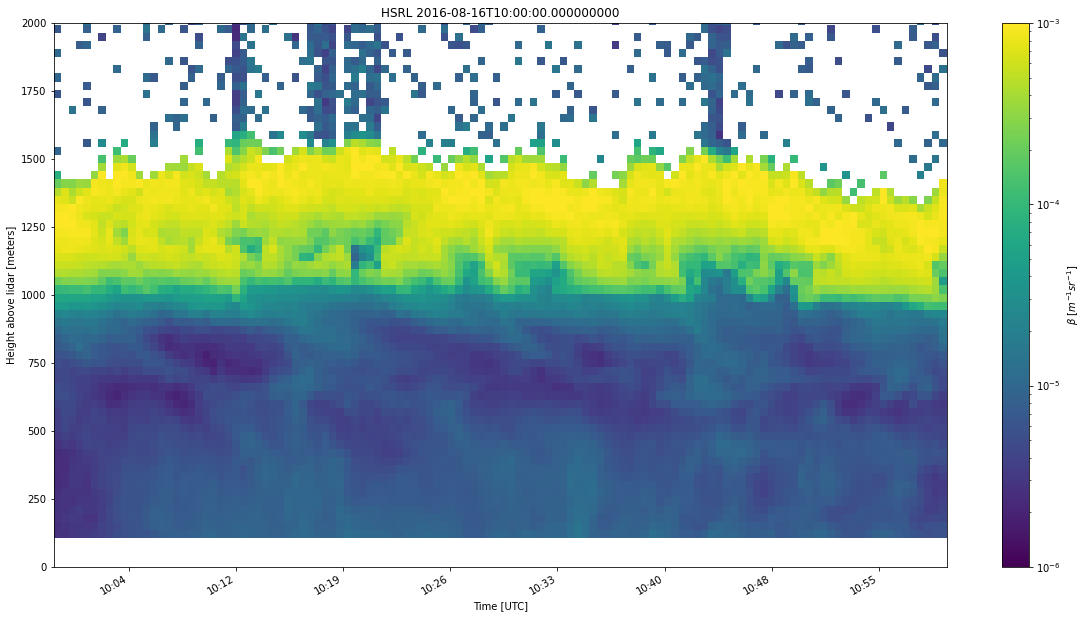
[8]:
model_display = emc2.plotting.SubcolumnDisplay(my_model, figsize=(20, 10))
ax_mod, _ = model_display.plot_subcolumn_timeseries("sub_col_beta_p_tot", 0, log_plot=True, y_range=(0., 2000.),
                                                 pressure_coords=False, cmap="viridis", vmin=1e-6, vmax=1e-3)
ax_mod.xaxis.set_major_formatter(mdates.DateFormatter('%H:%M'))
display.fig.savefig('HSRL_backscatter_simulated.png', dpi=200)
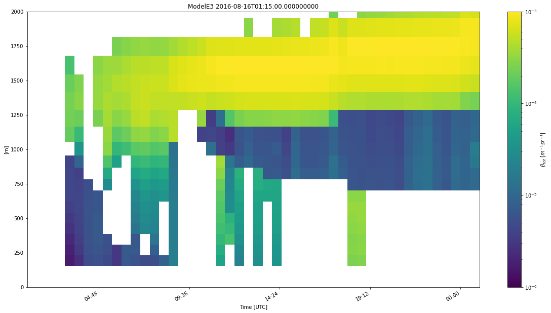
We can also use \(EMC^2\)’s SubcolumnDisplay object to generate profile plots with shaded regions designating variable temporal or spatial (based on all subcolumns) standard deviation.
[9]:
model_display_prof = emc2.plotting.SubcolumnDisplay(my_model, figsize=(5,8))
axp = model_display_prof.plot_subcolumn_mean_profile("sub_col_beta_p_tot", "2016-08-16T10:00:00", log_plot=True,
                                                     y_range=(0., 2000.), x_range=(1e-6, 1e-3), color='black',
                                                     pressure_coords=False, alpha=0.2)
axp = model_display_prof.plot_instrument_mean_profile(HSRL, "beta_a_backscat", log_plot=True,
                                                     Mask_array=HSRL.ds["od_aerosol"] > 4.,
                                                     y_range=(0., 2000.), x_range=(1e-6, 1e-3), color="lime",
                                                     pressure_coords=False, alpha=0.2)
display.fig.savefig('HSRL_backscatter_simulated_profile.png', dpi=200)
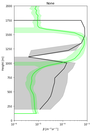
Finally, \(EMC^2\)’s SubcolumnDisplay object also allows easy production of phase classification plots. Here we demonstrate curtain plots of lidar classificaiton for the first subcolumn and frequency phase ratio calculated using all subcolumn data.
[10]:
model_display2 = emc2.plotting.SubcolumnDisplay(my_model, figsize=(20,10), subplot_shape=(2, 1))
ax2_1, cb2_1 = model_display2.plot_subcolumn_timeseries("phase_mask_HSRL_all_hyd", 0, y_range=(0., 2000.),
                                                 pressure_coords=False, subplot_index=0)
model_display.change_plot_to_class_mask(cb2_1, variable="phase_mask_HSRL_all_hyd", convert_zeros_to_nan=True)
ax2_1.xaxis.set_major_formatter(mdates.DateFormatter('%H:%M'))

my_model = emc2.simulator.classification.calculate_phase_ratio(my_model, "phase_mask_HSRL_all_hyd", [1])
ax2_2, cb2_2 = model_display2.plot_subcolumn_timeseries("phase_mask_HSRL_all_hyd_fpr", 0, y_range=(0., 2000.),
                                                    pressure_coords=False, cmap="bwr", subplot_index=1,
                                                    cbar_label='Frequency pr (reddish - more liquid)')
ax2_2.xaxis.set_major_formatter(mdates.DateFormatter('%H:%M'))
display.fig.savefig('HSRL_backscatter_simulated_class.png', dpi=200)